1   Preliminaries

1.1   Introduction

diagrams is a flexible, powerful embedded domain-specific language (EDSL) for creating vector graphics and animations. The diagrams framework is:

  • Declarative: you specify what a diagram is, not how to draw it. diagrams takes care of the how.

  • Compositional: diagrams can be easily combined in many ways to produce more complex diagrams.

  • Embedded: the full power of Haskell, including every library on Hackage, is available to help construct and manipulate graphics.

  • Extensible: extending diagrams with additional or higher-level functionality is as simple as writing a Haskell module.

  • Flexible: diagrams is designed from the ground up to be as generic and flexible as possible, with support for pluggable rendering backends, arbitrary graphics primitives, multiple numeric types, and multiple vector spaces (2D, 3D, ...).

1.2   About this document

This document attempts to explain all major aspects of using the diagrams core and standard libraries, organized by topic to make it easy to find what you are looking for. It is not, however, a complete reference of every single function in the standard library: for that, see the API documentation listed under Other resources. Most sections contain links to relevant modules you can follow to read about other functions not covered in the text.

Module names in the text are typeset like this: Diagrams.Prelude. Mathematical equations are typeset using MathJax:

\[\sum_{k=1}^\infty \frac{1}{k^2} = \frac{\pi^2}{6}\]

Right-click on any equation to access MathJax options, like displaying the LaTeX source, switching between MathML and HTML/CSS for display, zoom settings, and so on.

Occasionally content may be missing or incomplete; this is noted by a light blue box with a "document" icon on the right hand side, like this:

  • Explain zygohistomorphic prepromorphisms

  • Essay on postmodernist critiques of diagrams vis-a-vis Kant

If you see a box like this in the place of something you would really like to know about, please bug the developers (using the #diagrams IRC channel on Libera.Chat, or the diagrams mailing list) so they can prioritize it!

Warnings, "gotchas", and other important asides are in a yellow box with a "warning" icon, like this:

Diagrams is extremely addictive and may be hazardous to your health!

You would do well to pay special attention to the contents of such boxes.

1.3   Other resources

Here are some other resources that may be helpful to you as you learn about diagrams:

1.4   Installation

To use diagrams, you will need the following:

If you do not already have these, we recommend installing them via ghcup.

It is also easy to work with diagrams using stack, although that is not covered here.

No special installation step is actually needed — cabal or stack will automatically download and install the necessary diagrams packages for your project. For a minimal project you will need to depend on diagrams-lib (standard primitives and combinators) and a backend such as diagrams-svg. Optionally you may also depend on other packages in the diagrams ecosystem such as diagrams-contrib, SVGFonts, or palette.

There are several other Haskell-native backends including a postscript backend, which supports all features except transparency, and a raster backend (based on the excellent Rasterific package).

There is also a backend based on the cairo graphics library; it has support for more features than the SVG backend and additional output formats (PNG, PS, PDF), but can be much more difficult to install on some platforms (notably OS X).

There are other backends as well; see Rendering backends.

1.5   Getting started

Create a file called TestDiagram.hs (or whatever you like) with the following contents:

> {-# LANGUAGE NoMonomorphismRestriction #-}
> {-# LANGUAGE FlexibleContexts          #-}
> {-# LANGUAGE TypeFamilies              #-}
> 
> import Diagrams.Prelude
> import Diagrams.Backend.SVG.CmdLine
> -- or:
> -- import Diagrams.Backend.xxx.CmdLine
> -- where xxx is the backend you would like to use.
> 
> myCircle :: Diagram B
> myCircle = circle 1
> 
> main = mainWith myCircle

The first line turns off the dreaded monomorphism restriction, which is quite important when using diagrams: otherwise you will probably run into lots of crazy error messages.

The other two extensions are not needed for this simple example in particular, but are often required by diagrams in general, so it doesn't hurt to include them as a matter of course.

Diagrams.Prelude re-exports almost everything from the diagrams standard library, along with things from other packages which are often used in conjunction with diagrams. Diagrams.Backend.SVG.CmdLine provides a command-line interface to the SVG rendering backend. We then declare myCircle to have the type Diagram B. The B is an alias representing the particular backend. All backends export B as an alias for themselves, so you can switch backends just by changing an import, without having to change type annotations on your diagrams; B simply refers to whichever backend is in scope. Finally, mainWith takes a diagram and creates a command-line-driven executable for rendering it. GHC needs some help to determine the type of the argument of mainWith so it is important to annotate the type of myCircle (or whatever argument you pass to mainWith) as Diagram B.

Now create a simple test-diagram.cabal file (or similar) with the following contents:

cabal-version:      2.4
name:               test-diagram
version:            0.1.0.0
executable test-diagram
    main-is:          TestDiagram.hs
    build-depends:    base, diagrams-lib, diagrams-svg
    default-language: Haskell2010

You should now be able to build and run the example using the following commands:

$ cabal build
... lots of output while it downloads and builds all the dependencies ...

$ cabal exec test-diagram -- -w 100 -h 100 -o test-diagram.svg

(Note that the $ indicates a command prompt and should not actually be typed.) The above will generate a 100x100 SVG that should look like this:

If you are using the rasterific backend you can also request a .png, .jpg, .tif, or .bmp file (the format is automatically determined by the extension), or an .eps file if using the postscript backend. The cairo backend allows .svg, .png, .ps, and .pdf.

Try typing

$ cabal exec test-diagram -- --help

to see the other options that are supported.

To get started quickly, you may wish to continue by reading the quick start tutorial; or you can continue reading the rest of this user manual.

Note that Diagrams.Backend.SVG.CmdLine is provided for convenience, but it is not the only interface to the backend. For more control over when and how diagrams are rendered, e.g. as one component of a larger program, use the renderDia function, or see the related section under Rendering backends for additional backend specific entry points.

1.6   Contributing

diagrams is an open-source project, and contributions are encouraged! All diagrams-related repositories are in the diagrams organization on github. The Contributing page on the diagrams wiki explains how to get the repositories and make contributions. To find out about the latest developments, join the #diagrams IRC channel on Libera.Chat, and check out the diagrams Trello board.

2   Essential concepts

Before we jump into the main content of the manual, this chapter explains a number of general ideas and central concepts that will recur throughought. If you're eager to skip right to the good stuff, feel free to skip this section at first, and come back to it when necessary; there are many links to this chapter from elsewhere in the manual.

2.1   Semigroups and monoids

A semigroup consists of

  • A set of elements \(S\)

  • An associative binary operation on the set, that is, some operation

    \[\diamond \colon S \to S \to S\]

    for which

    \[(x \diamond y) \diamond z = x \diamond (y \diamond z).\]

A monoid is a semigroup with the addition of

  • An identity element \(i \in S\) which is the identity for \(\diamond\), that is,

    \[x \diamond i = i \diamond x = x.\]

In Haskell, semigroups are expressed using the Semigroup type class from the semigroups package:

> class Semigroup s where
>   (<>) :: s -> s -> s

and monoids are expressed using the Monoid type class, defined in Data.Monoid:

> class Monoid m where
>   mempty  :: m
>   mappend :: m -> m -> m

The mappend function represents the associative binary operation, and mempty is the identity element. (mappend and (<>) should always be the same; there are two different functions for historical reasons.) A function

> mconcat :: Monoid m => [m] -> m

is also provided as a shorthand for the common operation of combining a whole list of elements with (<>)/mappend.

Semigroups and monoids are used extensively in diagrams: diagrams, transformations, envelopes, traces, trails, paths, styles, colors, and queries are all instances of both Semigroup and Monoid.

2.2   Faking optional named arguments

Many diagram-related operations can be customized in a wide variety of ways. For example, when creating a regular polygon, one can customize the number of sides, the radius, the orientation, and so on. However, to have a single function that takes all of these options as separate arguments would be a real pain: it's hard to remember what the arguments are and what order they should go in, and often one wants to use default values for many of the options and only override a few. Some languages (such as Python) support optional, named function arguments, which are ideal for this sort of situation. Sadly, Haskell does not. However, we can fake it!

Any function which should take some optional, named arguments instead takes a single argument which is a record of options. The record type is declared to be an instance of the Default type class:

> class Default d where
>   def :: d

That is, types which have a Default instance have some default value called def. For option records, def is declared to be the record containing all the default arguments. The idea is that you can pass def as an argument to a function which takes a record of options, and override only the fields you want, like this:

> foo (def & arg1 .~ someValue & arg6 .~ blah)

This is using machinery from the lens package; but you don't have to understand lens, or know anything beyond the above syntax in order to use diagrams (for convenience, diagrams re-exports the (&) and (.~) operators from lens). In fact, in most cases, you can also use record update syntax instead (note the underscores):

foo (def { _arg1 = someValue, _arg6 = blah })

In some cases, however, the lens library is used to provide convenient "virtual" fields which do not correspond to real record fields; for example, headColor can be used to set the color of an arrowhead, even though the arrow options record actually contains a general style instead of just a color.

Finally, note that diagrams also defines with as a synonym for def, which can read a bit more nicely. So, instead of the above, you could write

foo (with & arg1 .~ someValue & arg6 .~ blah)

Most functions which take an optional arguments record have two variants: one named foo which uses all default arguments, and one named foo' (with a trailing prime) which takes an options record.

2.3   Postfix transformation

You will often see idiomatic diagrams code that looks like this:

foobar # attr1
       # attr2
       # attr3
       # transform1

There is nothing magical about (#), and it is not required in order to apply attributes or transformations. In fact, it is nothing more than reverse function application with a high precedence (namely, 8):

infixl 8 #
x # f = f x

(#) is provided simply because it often reads better to first write down what a diagram is, and then afterwards write down attributes and modifications. Additionally, (#) has a high precedence so it can be used to make "local" modifications without requiring lots of parentheses:

> example =     square 2 # fc red # rotateBy (1/3)
>           ||| circle 1 # lc blue # fc green

Note how the modifiers fc red and rotateBy (1/3) apply only to the square, and lc blue and fc green only to the circle. The horizontal composition operator (|||) has a precedence of 6, lower than that of (#).

2.4   Vectors and points

Although much of this user manual focuses on constructing two-dimensional diagrams, the definitions in the core library in fact work for any vector space. Vector spaces are defined in the Linear.Vector module from Edward Kmett's linear package.

Many objects (diagrams, paths, backends...) inherently live in some particular vector space. The vector space in which a given type "lives" can be computed by the type function Vn. So, for example, the type

Foo d => Vn d -> d -> d

is the type of a two-argument function whose first argument is a vector in whatever vector space corresponds to the type d (which must be an instance of Foo).

Each vector space has a dimension and a type of scalars. The type V2 Double specifies that the dimension is 2 and the scalar type is Double (64-bit floating point values). A vector represents a direction and magnitude, whereas a scalar represents only a magnitude. Useful operations on vectors and scalars include:

  • Adding and subtracting vectors with (^+^) and (^-^)

  • Multiplying a vector by a scalar with (*^)

  • Linearly interpolating between two vectors with lerp

  • Finding the norm (length) of a vector

  • Projecting one vector onto another with project.

Functions and types which are parametric in the vector space have two type parameters, v representing the dimension and n the scalar type. Occasionally v or n appears alone in a type signature, with the same meaning. n is most commonly Double, or some other type approximating the real numbers, but this is not required. Many functions require that n be an instance of Num, or one of the narrower classes Fractional, Floating, or Real.

See this tutorial for a more in-depth introduction to working with vectors and points.

One might think we could also identify points in a space with vectors having one end at the origin. However, this turns out to be a poor idea. There is a very important difference between vectors and points: namely, vectors are translationally invariant whereas points are not. A vector represents a direction and magnitude, not a location. Translating a vector has no effect. Points, on the other hand, represent a specific location. Translating a point results in a different point.

Although it is a bad idea to conflate vectors and points, we can certainly represent points using vectors. The linear package defines a newtype wrapper around vectors called Point. The most important connection between points and vectors is given by (.-.), defined in Linear.Affine. If p and q are points, q .-. p is the vector giving the direction and distance from p to q. Offsetting a point by a vector (resulting in a new point) is accomplished with (.+^).

2.5   Envelopes and local vector spaces

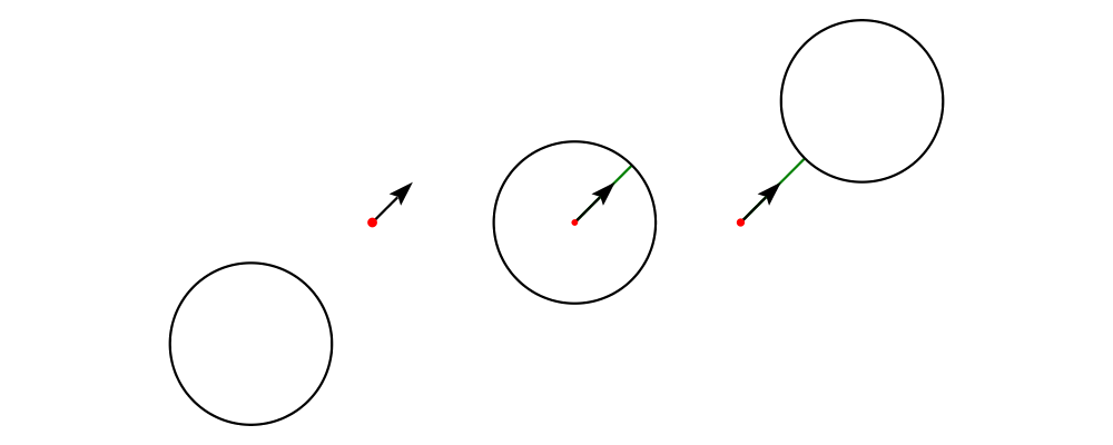
In order to be able to position diagrams relative to one another, each diagram must keep track of some bounds information. Rather than use a bounding box (which is neither general nor compositional) or even a more general bounding path (which is rather complicated to deal with), each diagram has an associated bounding function, called the envelope. Given some direction (represented by a vector) as input, the envelope answers the question: "how far in this direction must one go before reaching a perpendicular (hyper)plane that completely encloses the diagram on one side of it?"

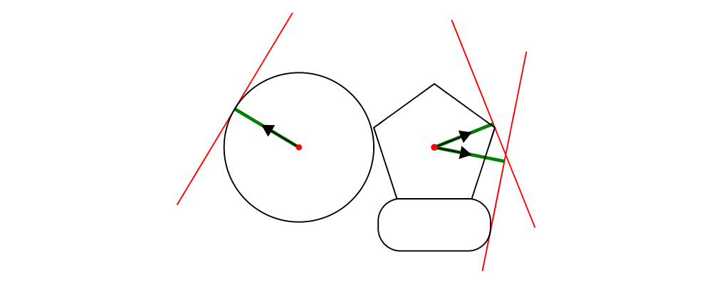
That's a bit of a mouthful, so hopefully the below illustration will help clarify things if you found the above description confusing. (For completeness, the code used to generate the illustration is included, although you certainly aren't expected to understand it yet if you are just reading this manual for the first time!)

> illustrateEnvelope v d
>   = mconcat
>     [arrowAt' (with & arrowHead .~ tri) origin v
>     , origin ~~ b
>       # lc green # lw veryThick
>     , p1 ~~ p2
>       # lc red
>     ]
>     where
>       b  = envelopeP v d
>       v' = 1.5 *^ signorm v
>       p1 = b .+^ (rotateBy (1/4) v')
>       p2 = b .+^ (rotateBy (-1/4) v')
>
> d1 :: Path V2 Double
> d1 = circle 1
>
> d2 :: Path V2 Double
> d2 = (pentagon 1 === roundedRect 1.5 0.7 0.3)
>
> example = (stroke d1 # showOrigin <> illustrateEnvelope (r2 (-0.5, 0.3)) d1)
>       ||| (stroke d2 # showOrigin <> illustrateEnvelope (r2 (0.5, 0.2)) d2
>                                   <> illustrateEnvelope (r2 (0.5, -0.1)) d2
>           )

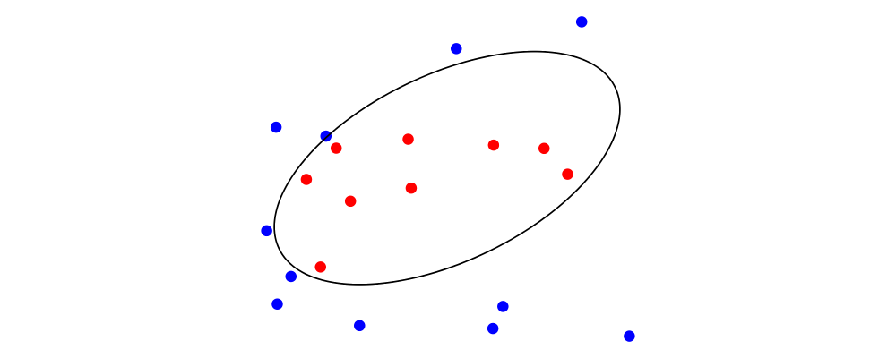
The black arrows represent inputs to the envelopes for the two diagrams; the envelopes' outputs are the distances represented by the thick green lines. The red lines illustrate the enclosing (hyper)planes (which are really to be thought of as extending infinitely to either side): notice how they are as close as possible to the diagrams without intersecting them at all.

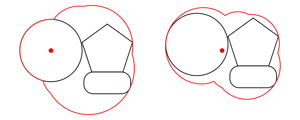
Of course, the base point from which the envelope is measuring matters quite a lot! If there were no base point, questions of the form "how far do you have to go..." would be meaningless—how far from where? This base point (indicated by the red dots in the diagram above) is called the local origin of a diagram. Every diagram has its own intrinsic local vector space; operations on diagrams are always with respect to their local origin, and you can affect the way diagrams are combined with one another by moving their local origins. The showOrigin function is provided as a quick way of visualizing the local origin of a diagram (also illustrated above). The showEnvelope method can also be used to show (an approximation of) the envelope of a diagram. For example:

> d1, d2 :: Diagram B
> d1 = circle 1
> d2 = (pentagon 1 === roundedRect 1.5 0.7 0.3)
>
> example = hsep 1
>   [ (d1 ||| d2)          # showEnvelope' (with & ePoints .~ 360) # showOrigin
>   , (d1 ||| d2) # center # showEnvelope' (with & ePoints .~ 360) # showOrigin
>   ]

As you can see, the location of the origin can make a big difference!

2.6   Measurement units

Certain attributes (such as line width, dashing size, arrowhead size, and font size) can be specified with respect to several different reference frames. For example, the lines used to draw a certain square can be specified as an absolute two pixels wide, or as a certain percentage of the size of the final diagram, or in units relative to the size of the square. More specifically, values of type Measure n represent n values, interpreted in one of four "reference frames": local, global, normalized, or output, described below in turn.

In addition to the four reference frames described here, it is possible to combine them into more complex expressions using a small DSL for specifying measurements; see Measurement expressions.

Local units

local units are the most straightforward to explain. Values in local units are interpreted in the context of the local vector space, just as most other length measurements (e.g. arguments to functions like circle and square). For example, square 1 # lwL 0.2 specifies a square which is drawn with lines one fifth as wide as its sides are long—and will always be, even if it is scaled: the line width scales right along with the square. (The L in lwL stands for "Local".)

> localSq = square 1 # lwL 0.2
> example =
>   hsep 0.5
>   [localSq, localSq # scale 2, localSq # scaleX 2]

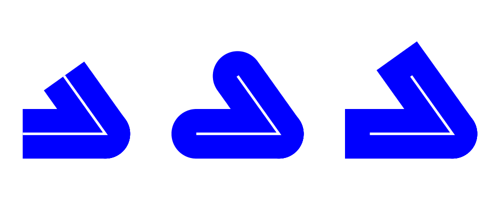
It's important to note that—as illustrated by the third figure in the above picture—line width always scales uniformly, even when a non-uniform scaling is applied. That is, the line used to draw the rectangle in the example above is a uniform thickness all the way around. Previous versions of diagrams had a freeze operation which could be used to apply non-uniform scaling to lines; to achieve such an effect, you can first turn a stroked line into a closed path, as described in Offsets of segments, trails, and paths.

A important consequence of local units having the current vector space as their reference is that attribute-setting functions such as lwL do not commute with transformations.

> example =
>   hsep 0.5
>   [ square 1 # lwL 0.2 # scale 2
>   , square 1 # scale 2 # lwL 0.2
>   ]
>   # frame 0.5

Global units

Whereas local values are interpreted in the current, "local" vector space, global values are interpreted in the final, "global" vector space of the diagram that is rendered. In the following example, theSq is specified as having a global line width of 0.05; five differently-scaled copies of the square are laid out, so that the entire scaled diagram has a width of around 6 units. The lines, having a line width of global 0.05, are thus about 0.8% of the width of the entire diagram.

> theSq = square 1 # lwG 0.05
>
> example =
>   hsep 0.2
>     (map (\s -> theSq # scale s) [0.5, 0.8, 1, 1.5, 2])

Versions of diagrams prior to 1.2 actually had a semantics for lw equivalent to lwG. One advantage, as can be seen from the above example, is that different shapes having the same global line width, even when differently scaled, will all be drawn with the same apparent line width. However, normalized and output have that property as well, and are probably more useful; the problem with global units is that in order to decide on values, one has to know the final size of the diagram, which is not typically something one knows in advance. In particular, note that applying something like scale 20 to the example above—a seemingly innocuous change—would result in extremely thin lines (or even invisible, depending on the backend), as shown below. Making this look reasonable again would require changing the argument to lwG.

> theSq = square 1 # lwG 0.05
>
> example =
>   hsep 0.2
>     (map (\s -> theSq # scale s) [0.5, 0.8, 1, 1.5, 2])
>   # scale 20

In short, global units tend to go against diagrams emphasis on local, scale-invariant thinking. They were left in for backwards compatibility, and because they can occasionally be useful in special situations where you do already have some absolute, global coordinate system in mind: for example, if you know you want to construct a 100x100 diagram using lines that are 1 unit wide.

Normalized units

normalized units, like global units, are measured with respect to the final size of a diagram. However, for the purposes of interpreting normalized units, the diagram is considered to be one "normalized unit" in both height and width. For example, a normalized value of 0.1 means "10% of the height/width of the final diagram". Thus, scaling the diagram has no effect on the relative size of the lines (just as with local), but lines look consistent even across shapes that have been scaled differently (as with global).

> theSq = square 1 # lwN 0.01
>
> example =
>   hsep 0.2
>     (map (\s -> theSq # scale s) [0.5, 0.8, 1, 1.5, 2])
>   # scale 20

Note that the scale 20 threatened in the global example has been applied here, but makes no difference: changing the 20 to any other nonzero value has no effect on the appearance of the rendered diagram.

Output units

Values measured in output units are interpreted with respect to the requested output size of a diagram. Sometimes you really do know, for example, that you want your lines to be exactly 1/2 inch wide when printed, or exactly 4 pixels wide on the screen. In this case, scaling a diagram will preserve its appearance, but requesting a different output size might not.

One situation in which output units can be particularly useful is when preparing a document (paper, blog post, etc.) with multiple embedded diagrams of various physical sizes. Using the same output value for the line width (or arrowhead length, arrow gap, font size, etc.) of every diagram ensures that the diagrams will all look consistent. (The default for line width is to use normalized units, but this means that by default, lines will only look consistent across multiple diagrams if all the diagrams have the same physical size, e.g. they are all \(300 \times 200\) pixels.)

> theSq = square 1 # lwO 4
>
> example =
>   hsep 0.2
>     (map (\s -> theSq # scale s) [0.5, 0.8, 1, 1.5, 2])
>   # scale 20

In the above example, all the squares are drawn with lines exactly 4 pixels wide (at least in theory; antialiasing makes the details a bit more subtle). Note that the actual units used (in this case, pixels) depends on the backend being used.

2.7   Types and type classes

Flexibility, power, simplicity: in general, you can have any two of these but not all three. Diagrams chooses flexibility and power, at the expense of simplicity. (In comparison, the excellent gloss library instead chooses flexibility and simplicity.) In particular, the types in the diagrams library can be quite intimidating at first. For example, hcat is a function which takes a list of diagrams and lays them out in a horizontal row. So one might expect its type to be something like [Diagram] -> Diagram. In actuality, its type is

> hcat :: (Juxtaposable a, HasOrigin a, Monoid' a, V a ~ V2, N a ~ n, TypeableFloat n)
>    => [a] -> a

which may indeed be intimidating at first glance, and at any rate takes a bit of time and practice to understand! The essential idea is to realize that hcat is actually quite a bit more general than previously described: it can lay out not just diagrams, but any two-dimensional things (V a ~ V2 and the constraints on N a) which can be positioned "next to" one another (Juxtaposable), can be translated (HasOrigin), and are an instance of Monoid (Monoid' is actually a synonym for the combination of Monoid and Semigroup). This certainly includes diagrams, but it also includes other things like paths, envelopes, animations, and even tuples, lists, sets, or maps containing any of these things.

At first, you may want to just try working through some examples intuitively, without worrying too much about the types involved. However, at some point you will of course want to dig deeper into understanding the types, either to understand an error message (though for help interpreting some common error messages, see Deciphering error messages) or to wield diagrams like a true type ninja. When that point comes, you should refer to Understanding diagrams types and the Type class reference.

3   Creating 2D diagrams

The main purpose of diagrams is to construct two-dimensional vector graphics (although it can be used for more general purposes as well). This section explains the building blocks provided by diagrams-core and diagrams-lib for constructing two-dimensional diagrams.

All 2D-specific things can be found in Diagrams.TwoD, which re-exports most of the contents of Diagrams.TwoD.* modules. This section also covers many things which are not specific to two dimensions; later sections will make clear which are which.

3.1   Basic 2D types

Diagrams.TwoD.Types defines types for working with two-dimensional Euclidean space.

Euclidean 2-space

There are three main type synonyms defined for referring to two-dimensional space:

  • V2 n is the type of a two-dimensional Euclidean vector space (n is usually Double). Standard diagrams backends render images with the positive \(x\)-axis extending to the right, and the positive \(y\)-axis extending upwards. This is consistent with standard mathematical practice, but upside-down with respect to many common graphics systems. This is intentional: the goal is to provide an elegant interface which is abstracted as much as possible from implementation details.

    unitX and unitY are unit vectors in the positive \(x\)- and \(y\)-directions, respectively. Their negated counterparts are unit_X and unit_Y.

    Vectors of type V2 Double can be created by passing a pair of type (Double, Double) to the function r2; vectors can likewise be converted back into pairs using unr2.

    Vectors can also be constructed and pattern-matched using the utilities defined in Diagrams.Coordinates, which provides a uniform interface for constructing points and vectors of any dimension. Vectors can be created using the syntax (x ^& y) and pattern-matched by calling coords and then matching on the pattern (x :& y).

    For more in-depth information on working with V2 Double, see this tutorial.

  • P2 n is the type of points in two-dimensional space. It is a synonym for Point V2 n. The distinction between points and vectors is important; see Vectors and points.

    Points can be created from pairs of coordinates using p2 and converted back using unp2. They can also be constructed and destructed using the same syntax as for vectors, as defined in Diagrams.Coordinates.

    For more in-depth information on working with P2, see this tutorial.

  • T2 n is the type of two-dimensional affine transformations. It is a synonym for Transformation V2 n.

Angles

The type Angle n represents two-dimensional angles. Angles can be expressed in radians, degrees, or fractions of a circle. Isomorphisms turn, rad, and deg are provided (represented using the Iso type from the lens package), which convert between abstract Angle n values and n values with various units. To construct an Angle, use the (@@) operator, as in (3 @@ deg) or (3 @@ rad). To project an Angle back to a scalar, use the (^.) operator, as in someAngle ^. rad.

  • turn represents fractions of a circle. A value of 1 @@ turn represents a full turn, 1/4 @@ turn constructs a right angle, and so on. The measure of an Angle a in turns (represented with Double) can be obtained using a ^. turn.

  • rad represents angles measured in radians. A value of tau (that is, \(\tau = 2 \pi\)) represents a full turn. (If you haven't heard of \(\tau\), see The Tau Manifesto.)

  • deg represents angles measured in degrees. A value of 360 represents a full turn.

fullTurn :: Angle represents one full turn, equivalent to 1 @@ turn, tau @@ rad, or 360 @@ deg. halfTurn :: Angle is also provided for convenience.

There is no Num instance for Angle; this is intentional, since, for example, it is not clear what units would be used for a bare number used as an Angle, and multiplying two Angles is meaningless and should not be allowed. Angle does have an Additive instance, which means you can add and subtract angles using (^+^) and (^-^), and negate an angle with negated. The (*^), (^*), and (^/) operators can also be used to multiply or divide an Angle by a constant factor: for example, if theta :: Angle then theta ^/ 3 is the angle representing one-third of theta.

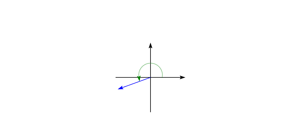
In two dimensions, the direction of a vector can be represented by an angle measured counterclockwise from the positive \(x\)-axis (shown in green below). For some vector u, this angle can be found by u ^. _theta.

Directions

Whereas a vector is described by a direction and a magnitude, some functions only depend on the direction. Direction v n is the type of directions of vectors of type v n; for example, Direction V2 Double represents directions in 2D Euclidean space. The direction function converts a vector to its Direction; fromDirection creates a unit (length 1) vector in the given direction.

xDir and yDir are provided as the directions of the positive x- and y-axes, respectively.

The relationship between Angles and Directions is similar to that between vectors and points, though unfortunately there cannot be a law-abiding Affine instance.

  • The Angle between two fixed Directions can be found with angleBetweenDirs, which is commutative and returns a positive angle between \(0\) and \(1/2\) turn, or signedAngleBetweenDirs, which satisfies signedAngleBetweenDirs d1 d2 == negated (signedAngleBetweenDirs d2 d1) and returns a positive angle when the second direction is clockwise from the first.

  • An Angle can be "added" to a Direction by simply using rotate to rotate the Direction by the Angle.

3.2   Primitive shapes

diagrams-lib provides many standard two-dimensional shapes for use in constructing diagrams.

Circles and ellipses

Circles can be created with the unitCircle and circle functions, defined in Diagrams.TwoD.Ellipse.

For example,

> example = circle 0.5 <> unitCircle

unitCircle creates a circle of radius 1 centered at the origin; circle takes the desired radius as an argument.

Every ellipse is the image of the unit circle under some affine transformation, so ellipses can be created by appropriately scaling and rotating circles.

> example = unitCircle # scaleX 0.5 # rotateBy (1/6)

For convenience the standard library also provides ellipse, for creating an ellipse with a given eccentricity, and ellipseXY, for creating an axis-aligned ellipse with specified radii in the x and y directions.

Arcs

Diagrams.TwoD.Arc provides a function arc, which constructs a radius-one circular arc starting at a first direction and extending through a given angle , as well as wedge which constructs a wedge shape with a given radius, annularWedge which expects an outer and inner radius, and various other functions for conveniently constructing arcs.

> example = hsep 0.5 [arc d a, wedge 1 d a, annularWedge 1 0.6 d a]
>   where
>     d :: Direction V2 Double
>     d = rotateBy (1/4) xDir
>     a :: Angle Double
>     a = (4 * tau / 7 - tau / 4) @@ rad

(Note that the parentheses in the definition of a are not strictly necessary, as (@@) has lower precedence (namely, 5) than (-) (which has precedence 6).)

Pre-defined shapes

Diagrams.TwoD.Shapes provides a number of pre-defined polygons and other path-based shapes. For example:

  • triangle constructs an equilateral triangle with sides of a given length.

  • square constructs a square with a given side length; unitSquare constructs a square with sides of length 1.

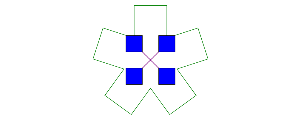
  • pentagon, hexagon, ..., dodecagon construct other regular polygons with sides of a given length. (For constructing polygons with a given radius, see General polygons.)

  • In general, regPoly constructs a regular polygon with any number of sides.

  • rect constructs a rectangle of a given width and height.

  • roundedRect constructs a rectangle with circular rounded corners.

  • roundedRect' works like roundedRect but allowing a different radius to be set for each corner, using RoundedRectOpts.

> example = square 1
>       ||| rect 0.3 0.5
>       ||| triangle 1
>       ||| roundedRect  0.5 0.4 0.1
>       ||| roundedRect  0.5 0.4 (-0.1)
>       ||| roundedRect' 0.7 0.4 (with & radiusTL .~ 0.2
>                                      & radiusTR .~ -0.2
>                                      & radiusBR .~ 0.1)

Completing the hodgepodge in Diagrams.TwoD.Shapes for now, the functions hrule and vrule create horizontal and vertical lines of a given length, respectively.

> example = c ||| hrule 1 ||| c
>   where c = circle 1 <> vrule 2

General polygons

The polygon function from Diagrams.TwoD.Polygons can be used to construct a wide variety of polygons. Its argument is a record of optional parameters that control the generated polygon:

  • polyType specifies one of several methods for determining the vertices of the polygon:

    • PolyRegular indicates a regular polygon with a certain number of sides and a given radius.

      > example = p 6 ||| p 24
      >   where p n = polygon (with
      >                 & polyType .~ PolyRegular n 1 )
    • PolySides specifies the vertices using a list of external angles between edges, and a list of edge lengths. More precisely, the first edge length is between the first and second vertex, while the first external angle is between the first and second edge. In the example below, the first vertex is on the bottom right.

      > example = polygon ( with
      >   & polyType .~ PolySides
      >       [ 20 @@ deg, 90 @@ deg, 40 @@ deg, 100 @@ deg ]
      >       [ 1        , 5        , 2        , 4          ]
      >   )
    • PolyPolar specifies the vertices using polar coordinates: a list of central angles between vertices, and a list of vertex radii.

  • polyOrient specifies the PolyOrientation: the polygon can be oriented with an edge parallel to the \(x\)-axis (OrientH), with an edge parallel to the \(y\)-axis (OrientV), or with an edge perpendicular to any given vector. You may also specify that no special orientation should be applied, in which case the first vertex of the polygon will be located along the positive \(x\)-axis.

  • Additionally, a center other than the origin can be specified using polyCenter.

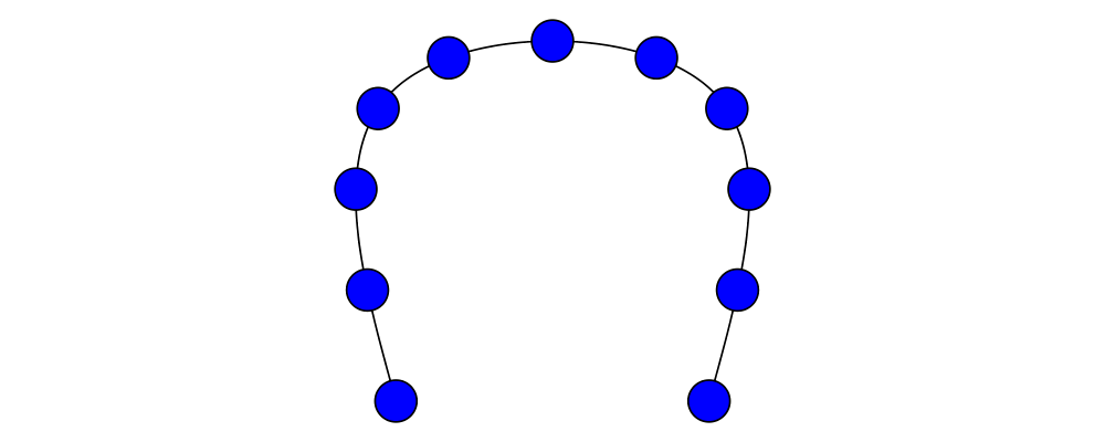
> poly1 = polygon ( with & polyType  .~ PolyRegular 13 5
>                        & polyOrient .~ OrientV )
> poly2 = polygon ( with & polyType  .~ PolyPolar (repeat (1/40 @@ turn))
>                                                 (take 40 $ cycle [2,7,4,6]) )
> example = (poly1 ||| strutX 1 ||| poly2)

Notice the idiom of using with to construct a record of default options and selectively overriding particular options by name. with is a synonym for def from the type class Default, which specifies a default value for types which are instances. You can read more about this idiom in the section Faking optional named arguments.

Star polygons

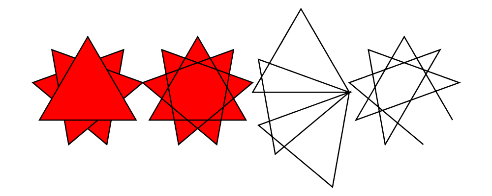
A "star polygon" is a polygon where the edges do not connect consecutive vertices; for example:

> example = star (StarSkip 3) (regPoly 13 1) # strokeP

Diagrams.TwoD.Polygons provides the star function for creating star polygons of this sort, although it is actually quite a bit more general.

As its second argument, star expects a list of points. One way to generate a list of points is with polygon-generating functions such as polygon or regPoly, or indeed, any function which can output any TrailLike type (see the section about TrailLike), since a list of points is an instance of the TrailLike class. But of course, you are free to construct the list of points using whatever method you like.

As its first argument, star takes a value of type StarOpts, for which there are two possibilities:

  • StarSkip specifies that every \(n\) th vertex should be connected by an edge.

    > example = strokeP (star (StarSkip 2) (regPoly 8 1))
    >       ||| strutX 1
    >       ||| strokeP (star (StarSkip 3) (regPoly 8 1))

    As you can see, star may result in a path with multiple components, if the argument to StarSkip and the number of vertices have a nontrivial common divisor.

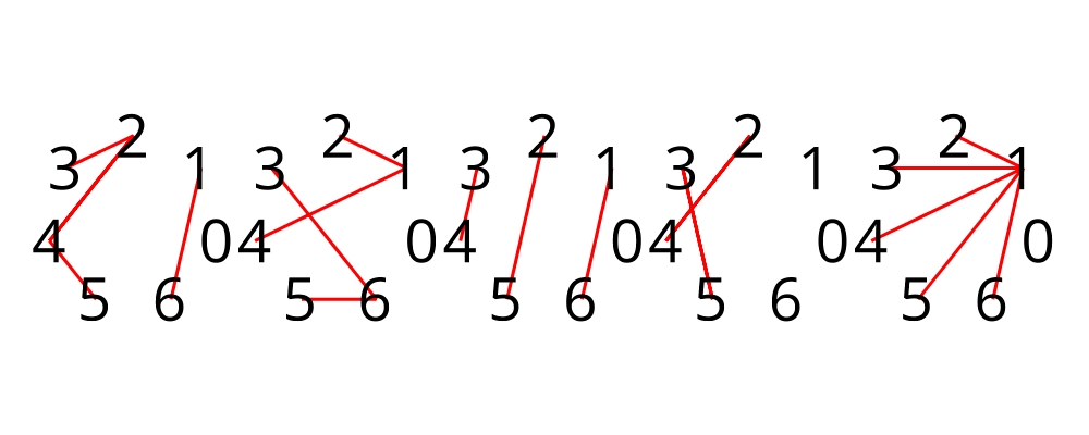
  • StarFun takes as an argument a function of type (Int -> Int), which specifies which vertices should be connected to which other vertices. Given the function \(f\), vertex \(i\) is connected to vertex \(j\) if and only if \(f(i) \equiv j \pmod n\), where \(n\) is the number of vertices. This can be used as a compact, precise way of specifying how to connect a set of points (or as a fun way to visualize functions in \(Z_n\)!).

    > {-# LANGUAGE MultiParamTypeClasses #-}
    > {-# LANGUAGE FlexibleContexts      #-}
    >
    > import Diagrams.TwoD.Text (Text)
    >
    > funs          = map (flip (^)) [2..6]
    > visualize :: (Int -> Int) -> Diagram B
    > visualize f   = strokeP' (with & vertexNames .~ [[0 .. 6 :: Int]] )
    >                     (regPoly 7 1)
    >                   # lw none
    >                   # showLabels
    >                   # fontSize (local 0.6)
    >              <> star (StarFun f) (regPoly 7 1)
    >                   # strokeP # lw thick # lc red
    > example       = center . hsep 0.5 $ map visualize funs

You may notice that all the above examples need to call strokeP (or strokeP'), which converts a path into a diagram. Many functions similar to star are polymorphic in their return type over any TrailLike, but star is not. As we have seen, star may need to construct a path with multiple components, which is not supported by the TrailLike class.

3.3   Composing diagrams

The diagrams framework is fundamentally compositional: complex diagrams are created by combining simpler diagrams in various ways. Many of the combination methods discussed in this section are defined in Diagrams.Combinators.

Superimposing diagrams with atop

The most fundamental way to combine two diagrams is to place one on top of the other with atop. The diagram d1 `atop` d2 is formed by placing d1's local origin on top of d2's local origin; that is, by identifying their local vector spaces.

> example = circle 1 `atop` square (sqrt 2)

As noted before, diagrams form a monoid with composition given by superposition. atop is simply a synonym for mappend (or (<>)), specialized to two dimensions.

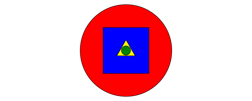
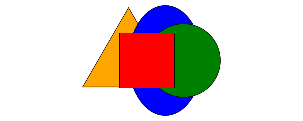
This also means that a list of diagrams can be stacked with mconcat; that is, mconcat [d1, d2, d3, ...] is the diagram with d1 on top of d2 on top of d3 on top of...

> example = mconcat [ circle 0.1 # fc green
>                   , triangle 1 # scale 0.4 # fc yellow
>                   , square 1   # fc blue
>                   , circle 1   # fc red
>                   ]

Juxtaposing diagrams

Fundamentally, atop is actually the only way to compose diagrams; however, there are a number of other combining methods (all ultimately implemented in terms of atop) provided for convenience.

Two diagrams can be placed next to each other using beside. The first argument to beside is a vector specifying a direction. The second and third arguments are diagrams, which are placed next to each other so that the vector points from the first diagram to the second.

> example = beside (r2 (20,30))
>                  (circle 1 # fc orange)
>                  (circle 1.5 # fc purple)
>           # showOrigin

As can be seen from the above example, the length of the vector makes no difference, only its direction is taken into account. (To place diagrams at a certain fixed distance from each other, see cat'.) As can also be seen, the local origin of the new, combined diagram is the same as the local origin of the first diagram. This makes beside v associative, so diagrams under beside v form a semigroup. In fact, they form a monoid, since mempty is a left and right identity for beside v, as can be seen in the example below:

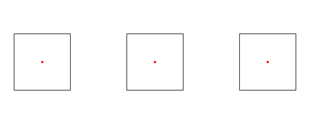
> example = hsep 1 . map showOrigin
>         $ [ d, mempty ||| d, d ||| mempty ]
>   where d = square 1

In older versions of diagrams, the local origin of the combined diagram was at the point of tangency between the two diagrams. To recover the old behavior, simply perform an alignment on the first diagram in the same direction as the argument to beside before combining (see Alignment):

> example = beside (r2 (20,30))
>                  (circle 1   # fc orange # align (r2 (20,30)))
>                  (circle 1.5 # fc purple)
>           # showOrigin

If you want to place two diagrams next to each other using the local origin of the second diagram, you can use something like beside' = flip . beside . negated, that is, use a vector in the opposite direction and give the diagrams in the other order.

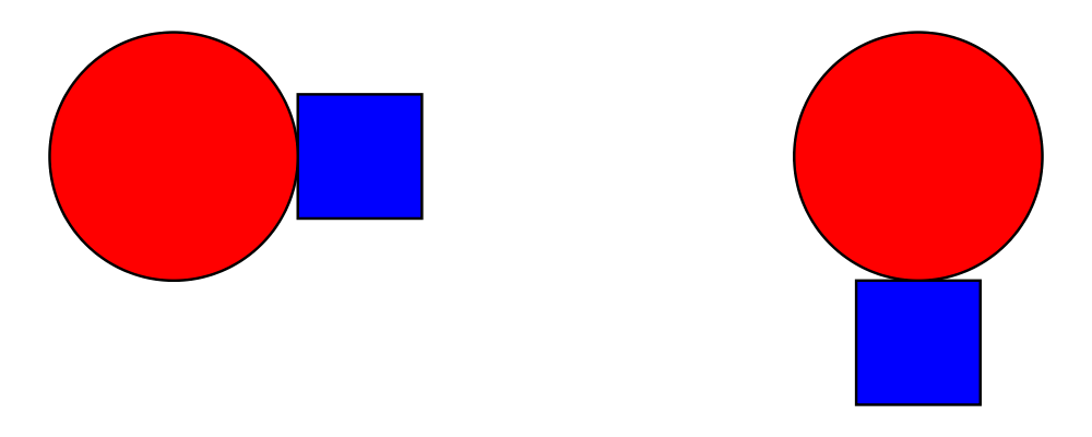
Since placing diagrams next to one another horizontally and vertically is quite common, special combinators are provided for convenience. (|||) and (===) are specializations of beside which juxtapose diagrams in the \(x\)- and \(y\)-directions, respectively.

> d1 = circle 1 # fc red
> d2 = square 1 # fc blue
> example = (d1 ||| d2) ||| strutX 3 ||| ( d1
>                                          ===
>                                          d2  )

Juxtaposing without composing

Sometimes, one may wish to position a diagram next to another diagram without actually composing them. This can be accomplished with the juxtapose function. In particular, juxtapose v d1 d2 returns a modified version of d2 which has been translated to be next to d1 in the direction of v. (In fact, beside itself is implemented as a call to juxtapose followed by a call to (<>).)

> d1 = juxtapose unitX             (square 1) (circle 1 # fc red)
> d2 = juxtapose (unitX ^+^ unitY) (square 1) (circle 1 # fc green)
> d3 = juxtapose unitY             (square 1) (circle 1 # fc blue)
> example = circles ||| strutX 1 ||| (circles <> square 1)
>   where circles = mconcat [d1, d2, d3]

See envelopes and local vector spaces for more information on what "next to" means, and Envelopes for information on functions available for manipulating envelopes. To learn about how envelopes are implemented, see the core library reference.

Concatenating diagrams

We have already seen one way to combine a list of diagrams, using mconcat to stack them. Several other methods for combining lists of diagrams are also provided in Diagrams.Combinators.

The simplest method of combining multiple diagrams is position, which takes a list of diagrams paired with points, and places the local origin of each diagram at the indicated point.

> example = position (zip (map mkPoint [-3, -2.8 .. 3]) (repeat spot))
>   where spot       = circle 0.2 # fc black
>         mkPoint x = p2 (x,x*x)

cat is an iterated version of beside, which takes a direction vector and a list of diagrams, laying out the diagrams beside one another in a row. The local origins of the subdiagrams will be placed along a straight line in the direction of the given vector, and the local origin of the first diagram in the list will be used as the local origin of the final result.

> example = cat (r2 (2, -1)) (map p [3..8]) # showOrigin
>   where p n = regPoly n 1

Semantically, cat v === foldr (beside v) mempty, although the actual implementation of cat uses a more efficient balanced fold.

For more control over the way in which the diagrams are laid out, use cat', a variant of cat which also takes a CatOpts record. See the documentation for cat' and CatOpts to learn about the various possibilities.

> example = cat' (r2 (2,-1)) (with & catMethod .~ Distrib & sep .~ 2 ) (map p [3..8])
>   where p n = regPoly n 1 # scale (1 + fromIntegral n/4)
>                           # showOrigin

For convenience, Diagrams.TwoD.Combinators also provides hcat, hcat', vcat, and vcat', variants of cat and cat' which concatenate diagrams horizontally and vertically. In addition, since using hcat' or vcat' with some separation tends to be common, hsep and vsep are provided as short synonyms; that is, hsep s = hcat' (with & sep .~ s), and similarly for vsep.

> example = hsep 0.2 (map square [0.3, 0.7 .. 2])

Finally, appends is like an iterated variant of beside, with the important difference that multiple diagrams are placed next to a single central diagram without reference to one another; simply iterating beside causes each of the previously appended diagrams to be taken into account when deciding where to place the next one. Of course, appends is implemented in terms of juxtapose (see Juxtaposing without composing).

> c        = circle 1
> dirs     = iterate (rotateBy (1/7)) unitX
> cdirs    = zip dirs (replicate 7 c)
> example1 = appends c cdirs
> example2 = foldl (\a (v,b) -> beside v a b) c cdirs
> example  = example1 ||| strutX 3 ||| example2

3.4   Modifying diagrams

Attributes and styles

Every diagram has a style which is an arbitrary collection of attributes. This section will describe some of the default attributes which are provided by the diagrams library and recognized by most backends. However, you can easily create your own attributes as well; for details, see the core library reference.

In many examples, you will see attributes applied to diagrams using the (#) operator. Keep in mind that there is nothing special about this operator as far as attributes are concerned. It is merely backwards function application, which is used for attributes since it often reads better to have the main diagram come first, followed by modifications to its attributes. See Postfix transformation.

In general, inner attributes (that is, attributes applied earlier) override outer ones. Note, however, that this is not a requirement. Each attribute may define its own specific method for combining multiple values. Again, see the core library reference for more details.

Most of the attributes discussed in this section are defined in Diagrams.TwoD.Attributes.

Texture

Two-dimensional diagrams can be filled and stroked with a Texture. A Texture can be either a solid color, a linear gradient or a radial gradient. Not all backends support gradients, in particular gradients are supported by the SVG, Cairo, and Rasterific backends (see Rendering backends). Future releases should also support patterns as textures. The data type for a texture is

> data Texture = SC SomeColor | LG LGradient | RG RGradient

and Prism s _SC, _LG, _RG are provided for access.

Color and Opacity

The color used to stroke the paths can be set with the lc (line color) function and the color used to fill them with the fc (fill color) function.

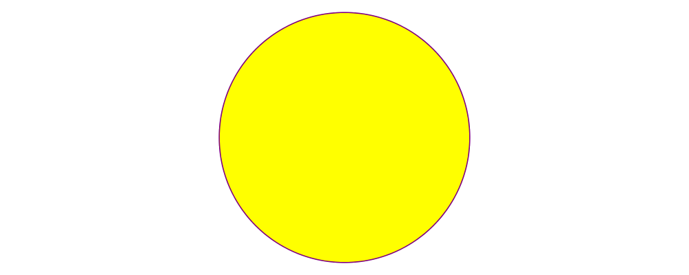
> example = circle 0.2 # lc purple # fc yellow

By default, diagrams use a black line color and a completely transparent fill color.

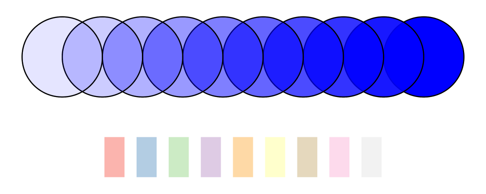
Colors themselves are handled by the colour package, which provides a large set of predefined color names as well as many more sophisticated color operations; see its documentation for more information. The colour package uses a different type for colors with an alpha channel (i.e. transparency). To make use of transparent colors you can use lcA and fcA. The palette package provides additional sets of colors and algorithms for creating harmonious color combinations.

> import Data.Colour (withOpacity)
> import Data.Colour.Palette.BrewerSet
>
> blues   = map (blue `withOpacity`) [0.1, 0.2 .. 1.0]
> alphaEx = hcat' (with & catMethod .~ Distrib & sep .~ 1 )
>                 (zipWith fcA blues (repeat (circle 1)))
>
> colors  = brewerSet Pastel1 9
> paletteEx = hsep 0.3 (zipWith fc colors (repeat (rect 0.5 1 # lw none)))
>
> example = vsep 1 ([alphaEx, paletteEx] # map centerX)

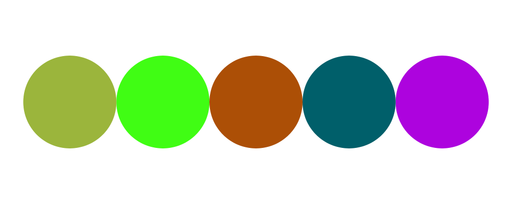
Another source of predefined color names is the Diagrams.Color.XKCD module, containing over 900 common names for colors as determined by the XKCD color name survey.

> import Diagrams.Color.XKCD
>
> colors = [booger, poisonGreen, cinnamon, petrol, vibrantPurple]
> example = hcat (zipWith fcA colors (repeat (circle 1 # lw none)))

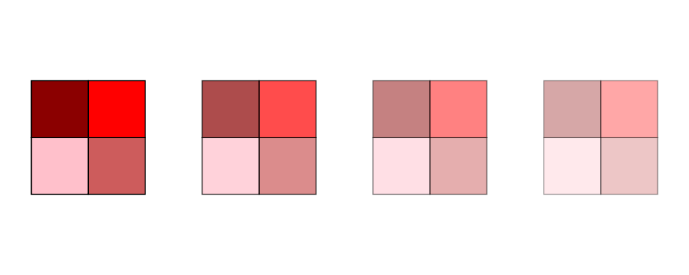
Transparency can also be tweaked with the Opacity attribute, which sets the opacity/transparency of a diagram as a whole. Applying opacity p to a diagram, where p is a value between 0 and 1, results in a diagram p times as opaque.

> s c     = square 1 # fc c
> reds    = (s darkred ||| s red) === (s pink ||| s indianred)
> example = hsep 1 . take 4 . iterate (opacity 0.7) $ reds

Some backends support setting fill and stroke opacities separately, with fillOpacity and strokeOpacity.

Grouped opacity can be applied using the opacityGroup annotation, which is currently supported by the diagrams-svg, diagrams-pgf, and (as of version 1.3.1) the diagrams-rasterific backends. In the example to the left below, the section where the two transparent circles overlap is darker, just as if e.g. two circles made out of colored cellophane were overlapped. If this documentation was compiled with a backend that supports opacity grouping (e.g. Rasterific or SVG), then the example on the right shows two transparent circles without a darker section where they overlap—the transparency has been applied to the group of diagrams as a whole, as if it were a single piece of cellophane cut in the shape of overlapping circles.

> cir = circle 1 # lw none # fc red
> overlap = (cir <> cir # translateX 1)
>
> example = hsep 1 [ overlap # opacity 0.3, overlap # opacityGroup 0.3 ]
>           # centerX
>        <> rect 9 0.1 # fc lightblue # lw none

To "set the background color" of a diagram, use the bg function—which does not actually set any attributes, but simply superimposes the diagram on top of a bounding rectangle of the given color. The bgFrame function is similar but the background is expanded to frame the diagram by a specified amount.

> t = regPoly 3 1
>
> example = hsep 0.2 [t, t # bg orange, t # bgFrame 0.1 orange]

Linear Gradients

A linear gradient must have a list of color stops, a starting point, an ending point, a transformation and a spread method. Color stops are pairs of (color, fraction) where the fraction is usually between 0 and 1 that are mapped onto the start and end points. The starting point and endping point are specified in local coordinates. Typically the transformation starts as the identity transform mempty and records any transformations that are applied to the object using the gradient. The spread method defines how space beyond the starting and ending points should be handled: GradPad will fill the space with the final stop color, GradRepeat will restart the gradient, and GradReflect will restart the gradient but with the stops reversed. This is the data type for a linear gradient:

> data LGradient n = LGradient
>   { _lGradStops        :: [GradientStop n]
>   , _lGradStart        :: P2 n,
>   , _lGradEnd          :: P2 n,
>   , _lGradTrans        :: T2 n,
>   , _lGradSpreadMethod :: SpreadMethod
>   }

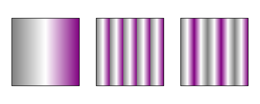
Lenses are provided to access the record fields. In addition the functions mkStops taking a list of triples (color, fraction, opacity) and mkLinearGradient which takes a list of stops, a start and end point, and a spread method and creates a Texture are provided for convenience. In this example we demonstrate how to make linear gradients with the mkLinearGradient functions and how to adjust it using the lenses and prisms.

> stops = mkStops [(gray, 0, 1), (white, 0.5, 1), (purple, 1, 1)]
> gradient = mkLinearGradient stops ((-0.5) ^& 0) (0.5 ^& 0) GradPad
> sq1 = square 1 # fillTexture  gradient
> sq2 = square 1 # fillTexture (gradient & _LG . lGradSpreadMethod .~ GradRepeat
>                                        & _LG . lGradStart        .~ (-0.1) ^& 0
>                                        & _LG . lGradEnd          .~ 0.1 ^& 0
>                              )
> sq3 = square 1 # fillTexture (gradient & _LG . lGradSpreadMethod .~ GradReflect
>                                        & _LG . lGradStart        .~ (-0.1) ^& 0
>                                        & _LG . lGradEnd          .~ 0.1 ^& 0
>                              )
>
> example = hsep 0.25 [sq1, sq2, sq3]

Here we apply the gradient to the stroke only and give it starting and ending points towards the corners.

> stops = mkStops [(teal, 0, 1), (orange, 1, 1)]
> gradient = mkLinearGradient stops ((-1) ^& (-1)) (1 ^& 1) GradPad
> example = rect 3 1 # lineTexture  gradient # lwO 15 # fc black # opacity 0.75

Radial Gradients

Radial gradients are similar, only they begin at the perimeter of an inner circle and end at the perimeter of an outer circle.

> data RGradient n = RGradient
>     { _rGradStops        :: [GradientStop n]
>     , _rGradCenter0      :: P2 n
>     , _rGradRadius0      :: n
>     , _rGradCenter1      :: P2 n
>     , _rGradRadius1      :: n
>     , _rGradTrans        :: T2 n
>     , _rGradSpreadMethod :: SpreadMethod }

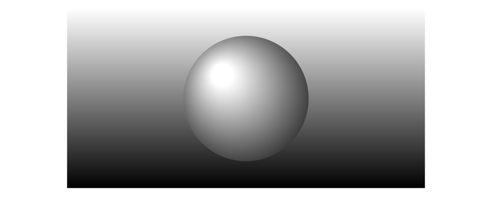
Where radius and center 0 are for the inner circle, and 1 for the outer circle. In this example we place the inner circle off center and place a circle filled with the radial gradient on top of a rectangle filled with a linear gradient to create a 3D effect.

> radial = mkRadialGradient (mkStops [(white,0,1), (black,1,1)])
>                           ((-0.15) ^& (0.15)) 0.06 (0 ^& 0) 0.5
>                           GradPad
>
> linear = mkLinearGradient (mkStops [(black,0,1), (white,1,1)])
>                           (0 ^& (-0.5)) (0 ^& 0.5)
>                           GradPad
>
> example = circle 0.35 # fillTexture radial # lw none
>        <> rect 2 1 # fillTexture linear # lw none

Line width

Line width is actually more subtle than you might think. Suppose you create a diagram consisting of a square, and another square twice as large next to it (using scale 2). How should they be drawn? Should the lines be the same width, or should the larger square use a line twice as thick? (Note that similar questions also come up when considering the dashing style used to draw some shapes—should the size of the dashes scale with transformations applied to the shapes, or not?) diagrams allows the user to decide, using Measure Double values to specify things like line width (see Measurement units).

In many situations, it is desirable to have lines drawn in a uniform way, regardless of any scaling applied to shapes. This is what happens with line widths measured in global, normalized or output units, as in the following example:

> example = hcat
>   [ square 1
>   , square 1 # scale 2
>   , circle 1 # scaleX 3
>   ]
>   # dashingN [0.03,0.03] 0
>   # lwN 0.01

For line widths that scale along with a diagram, use local; in this case line widths will be scaled in proportion to the geometeric average of the scaling transformations applied to the diagram.

The LineWidth attribute is used to alter the width with which paths are stroked. The most general functions that can be used to set the line width are lineWidth and its synonym lw, which take an argument of type Measure V2 n. Since typing things like lineWidth (normalized 0.01) is cumbersome, there are also shortcuts provided: lwG, lwN, lwO, and lwL all take an argument of type Double and wrap it in global, normalized, output and local, respectively.

There are also predefined Measure n values with intuitive names, namely, ultraThin, veryThin, thin, medium, thick, veryThick, ultraThick, and none (the default is medium), which should often suffice for setting the line width.

> line = strokeT . fromOffsets $ [unitX]
> example = vcat' (with & sep .~ 0.1)
>   [line # lw w | w <- [ultraThin, veryThin, thin,
>                        medium, thick, veryThick, ultraThick]]

In the above example, there is no discernible difference between ultraThin and veryThin (depending on the resolution of your display you may not see any difference with thin either); these names all describe normalized measurements with a physical lower bound, so the physical width of the resulting lines depends on the physical size of the rendered diagram. At larger rendering sizes the differences between the smaller widths become apparent.

Note that line width does not affect the envelope of diagrams at all. To stroke a line "internally", turning it into a Path value enclosing the stroked area (which does contribute to the envelope), you can use one of the functions described in the section Offsets of segments, trails, and paths.

Other line parameters

Many rendering backends provide some control over the particular way in which lines are drawn. Currently, diagrams provides built-in support for three aspects of line drawing:

  • lineCap sets the LineCap style.

  • lineJoin sets the LineJoin style.

  • dashing allows for drawing dashed lines with arbitrary dashing patterns.

> path = fromVertices (map p2 [(0,0), (1,0.3), (2,0), (2.2,0.3)]) # lwO 20
> example = center . vcat' (with & sep .~ 0.1 )
>           $ map (path #)
>             [ lineCap LineCapButt   . lineJoin LineJoinMiter
>             , lineCap LineCapRound  . lineJoin LineJoinRound
>             , lineCap LineCapSquare . lineJoin LineJoinBevel
>             , dashingN [0.03,0.06,0.09,0.03] 0
>             ]

The HasStyle class

Functions such as fc, lc, lw, and lineCap do not take only diagrams as arguments. They take any type which is an instance of the HasStyle type class. Of course, diagrams themselves are an instance.

However, the Style type is also an instance. This is useful in writing functions which offer the caller flexible control over the style of generated diagrams. The general pattern is to take a Style (or several) as an argument, then apply it to a diagram along with some default attributes:

> myFun style = d # applyStyle style # lc red # ...
>   where d = ...

This way, any attributes provided by the user in the style argument will override the default attributes specified afterwards.

To call myFun, a user can construct a Style by starting with an empty style (mempty, since Style is an instance of Monoid) and applying the desired attributes:

> foo = myFun (mempty # fontSize (local 2) # lw none # fc green)

If the type T is an instance of HasStyle, then [T] is also. This means that you can apply styles uniformly to entire lists of diagrams at once, which occasionally comes in handy, for example, to assign a default attribute to all diagrams in a list which do not already have one:

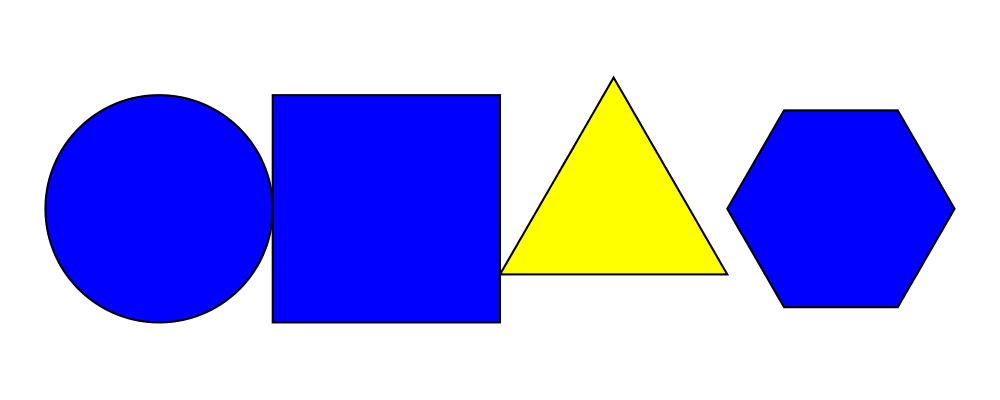
> example = hcat $
>   [circle 1, square 2, triangle 2 # fc yellow, hexagon 1] # fc blue

Likewise, there are HasStyle instances for pairs, Maps, Sets, and functions.

Static attributes

Diagrams can also have "static attributes" which are applied at a specific node in the tree representing a diagram. Currently, only two static attributes are provided:

  • Hyperlinks are supported only by the SVG backend. To turn a diagram into a hyperlink, use the href function.

  • Transparency grouping via the opacityGroup function is supported only by the SVG, PGF and (as of 1.3) Rasterific backends; see Color and Opacity.

More static attributes (for example, node IDs) and wider backend support may be added in future versions.

2D Transformations

Any diagram can be transformed by applying arbitrary affine transformations to it. Affine transformations include linear transformations (rotation, scaling, reflection, shears—anything which leaves the origin fixed and sends lines to lines) as well as translations. In the simplified case of the real line, an affine transformation is any function of the form \(f(x) = mx + b\). Generalizing to \(d\) dimensions, an affine transformation is a vector function of the form \(f(\mathbf{v}) = \mathbf{M}\mathbf{v} + \mathbf{b}\), where \(\mathbf{M}\) is a \(d \times d\) matrix representing a linear transformation, and \(\mathbf{b}\) is a \(d\)-dimensional vector representing a translation. More general, non-affine transformations, including projective transformations, are referred to in diagrams as Deformations.

Diagrams.TwoD.Transform defines a number of common affine transformations in two-dimensional space. (To construct transformations more directly, see Diagrams.Core.Transform.)

Every transformation comes in two variants, a noun form and a verb form. For example, there are two functions for scaling along the \(x\)-axis, scalingX and scaleX. The noun form (e.g. scalingX) constructs a Transformation value, which can then be stored in a data structure, passed as an argument, combined with other transformations, etc., and ultimately applied to a diagram (or other Transformable value) with the transform function. The verb form directly applies the transformation. The verb form is much more common (and the documentation below will only discuss verb forms), but getting one's hands on a first-class Transformation value can occasionally be useful.

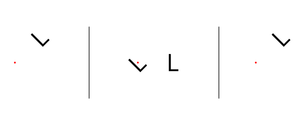
Both the verb and noun variants of transformations are monoids, and can be composed with (<>). However, the results are quite distinct, as shown in this example.

> ell = text "L" <> square 1 # lw none
> alpha = 45 @@ deg
>
> dia1 = ell # translateX 2 # rotate alpha
> dia2 = ell # ( rotate alpha <> translateX 2 )
> dia3 = ell # transform ( rotation alpha <> translationX 2 )
>
> example =
>   hsep 2
>     [ (dia1 <> orig)
>     , vrule 4
>     , (dia2 <> orig)
>     , vrule 4
>     , (dia3 <> orig)
>     ]
>   where
>     orig = circle 0.05 # fc red # lw none

dia1 is the intended result: a character L translated along the X axis, and then rotated 45 degrees around the origin.

dia2 shows the result of naively composing the verb versions of the transformations: a superposition of a rotated L and a translated L. To understand this, consider that (rotate alpha) is a function, and functions as monoid instances (Monoid m => Monoid (a -> m)) are composed as (f <> g) x = f x <> g x. To quote the Typeclassopedia: if a is a Monoid, then so is the function type e -> a for any e; in particular, g `mappend` h is the function which applies both g and h to its argument and then combines the results using the underlying Monoid instance for a.

Hence ell # ( rotate alpha <> translateX 2 ) is the same as the superposition of two diagrams: rotate alpha ell <> translateX 2 ell.

dia3 shows how the noun versions can be composed (using the Monoid instance for Transformation) with the intended result.

Affine transformations in general

Before looking at specific two-dimensional transformations, it's worth saying a bit about transformations in general (a fuller treatment can be found in the core library reference). The Transformation type is defined in Diagrams.Core.Transform, from the diagrams-core package. Transformation is parameterized by the vector space over which it acts, and the type of scalars; recall that T2 n is provided as a synonym for Transformation V2 n.

Transformation v n is a Monoid for any vector space v:

  • mempty is the identity transformation;

  • mappend is composition of transformations: t1 `mappend` t2 (also written t1 <> t2) performs first t2, then t1.

To invert a transformation, use inv. For any transformation t,

t <> inv t === inv t <> t === mempty.

To apply a transformation, use transform.

Rotation

Use rotate to rotate a diagram counterclockwise by a given angle about the origin. Since rotate takes an Angle n, you must specify an angle unit, such as rotate (80 @@ deg). In the common case that you wish to rotate by an angle specified as a certain fraction of a circle, like rotate (1/8 @@ turn), you can use rotateBy instead. rotateBy takes a Double argument expressing the number of turns, so in this example you would only have to write rotateBy (1/8).

You can also use rotateAbout in the case that you want to rotate about some point other than the origin.

> eff = text "F" <> square 1 # lw none
> rs  = map rotateBy [1/7, 2/7 .. 6/7]
> example = hcat . map (eff #) $ rs

Scaling and reflection

Scaling by a given factor is accomplished with scale (which scales uniformly in all directions), scaleX (which scales along the \(x\)-axis only), or scaleY (which scales along the \(y\)-axis only). All of these can be used both for enlarging (with a factor greater than one) and shrinking (with a factor less than one). Using a negative factor results in a reflection (in the case of scaleX and scaleY) or a 180-degree rotation (in the case of scale).

> eff = text "F" <> square 1 # lw none
> ts  = [ scale (1/2), id, scale 2,    scaleX 2,    scaleY 2
>       ,                  scale (-1), scaleX (-1), scaleY (-1)
>       ]
>
> example = hcat . map (eff #) $ ts

Scaling by zero is forbidden. Let us never speak of it again.

For convenience, reflectX and reflectY perform reflection along the \(x\)- and \(y\)-axes, respectively. Their names can be confusing (does reflectX reflect along the \(x\)-axis or across the \(x\)-axis?) but you can just remember that reflectX = scaleX (-1), and similarly for reflectY; that is, reflectQ affects Q-coordinates.

reflectXY swaps the \(x\)- and \(y\)-coordinates, that is, it reflects across the line \(y = x\). To reflect across any other line, use reflectAbout.

> eff = text "F" <> square 1 # lw none
> example = eff
>        <> reflectAbout (p2 (0.2,0.2)) (rotateBy (-1/10) xDir) eff

Translation

Translation is achieved with translate, translateX, and translateY, which should be self-explanatory.

Transformation matrices

Internally, diagrams does not use matrices to represent affine transformations, but Diagrams.Transform.Matrix provides several functions for converting back and forth between Transformations and their matrix representations.

Conjugation

Diagrams.Transform also exports some useful transformation utilities which are not specific to two dimensions. The conjugate function performs conjugation: conjugate t1 t2 == inv t1 <> t2 <> t1, that is, it performs t1, then t2, then undoes t1.

underT performs a transformation using conjugation. It takes as arguments a function f as well as a transformation to conjugate by, and produces a function which performs the transformation, then f, then the inverse of the transformation. For example, scaling by a factor of 2 along the diagonal line \(y = x\) can be accomplished thus:

> eff = text "F" <> square 1 # lw none
> example = (scaleX 2 `underT` rotation (-1/8 @@ turn)) eff

The letter F is first rotated so that the desired scaling axis lies along the \(x\)-axis; then scaleX is performed; then it is rotated back to its original position.

Note that reflectAbout and rotateAbout are implemented using underT.

Some functions for producing Isos (from the lens library) are also provided, which serve a similar purpose to conjugate and underT, but can be more convenient when working in a lens-y style. For example, the transformed function takes a Transformation and yields an Iso between untransformed and transformed things. movedTo, movedFrom, and translated work similarly, but specific to translation.

The Transformable class

Transformations can be applied not just to diagrams, but values of any type which is an instance of the Transformable type class. Instances of Transformable include vectors, points, trails, paths, envelopes, and Transformations themselves. In addition, tuples, lists, maps, or sets of Transformable things are also Transformable in the obvious way.

Deformations

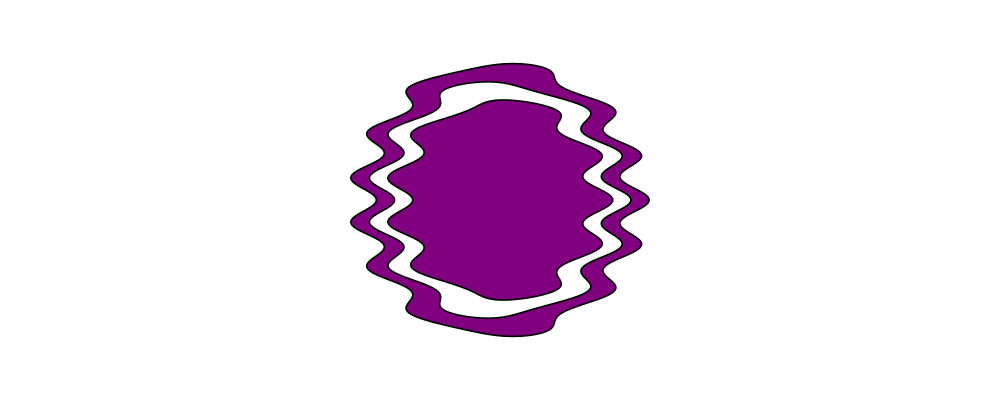
The affine transformations represented by Transformation include the most commonly used transformations, but occasionally other sorts are useful. Non-affine transformations are represented by the Deformation type. The design is quite similar to that of Transformation. A Deformation is parameterized by the vector spaces over which it acts: most generally, it may send objects in one vector space to objects in another. There is a Deformable type class with a function deform, which applies a Deformation to a Deformable value. There is also a function deform' which takes an extra tolerance parameter; applying deformations usually involves approximation.

> wibble :: Deformation V2 V2 Double
> wibble = Deformation $ \p ->
>   ((p^._x) + 0.3 * cos ((p ^. _y) * tau)) ^& (p ^. _y)
>   -- perturb x-coordinates by the cosine of the y-coordinate
>
> circles :: Path V2 Double
> circles = mconcat . map circle $ [3, 2.6, 2.2]
>
> example :: Diagram B
> example = circles # deform' 0.0001 wibble # strokeP
>         # fillRule EvenOdd # fc purple # frame 1

Because the deform function is so general, type signatures are often required on both its inputs and results, as in the example above; otherwise ambiguous type errors are likely to result.

Deformation v v n is a Monoid for any vector space v n. (In general, Deformation u v n maps objects with vector space u to ones with vector space v.) New deformations can be formed by composing two deformations. The composition of an affine transformation with a Deformation is also a Deformation. asDeformation converts a Transformation to an equivalent Deformation, "forgetting" the inverse and other extra information which distinguishes affine transformations.

The very general nature of deformations prevents certain types from being Deformable. Because not every Deformation is invertible, diagrams cannot be deformed. In general, for two points \(p\) and \(q\), and a deformation \(D\), there may be no deformation \(D_v\) such that \(Dp - Dq = D_v(p-q)\). For this reason, only points and concretely located types are deformable. Finally, segments are not deformable because the image of the segment may not be representable by a single segment. The Deformable instances for trails and paths will approximate each segment by several segments as necessary. Points, Located trails, and paths are all deformable.

Because approximation and subdivision are required for many Deformable instances, the type class provides a function deform', which takes the approximation accuracy as its first argument. For trails and paths, deform (without a prime) calls deform' with an error limit of 0.01 times the object's size.

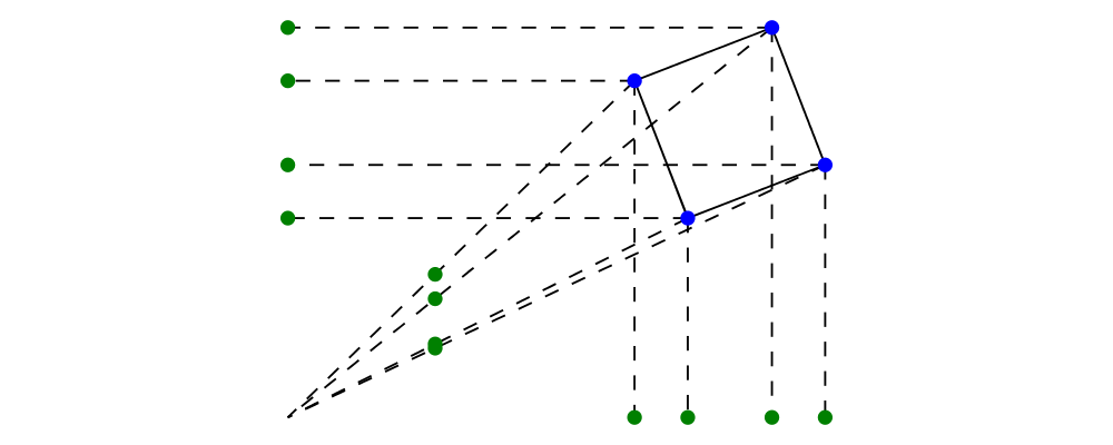
Diagrams.TwoD.Deform defines parallel and perspective projections along the principal axes in 2 dimensions. The below example projects the vertices of a square orthogonally onto the \(x\)- and \(y\)-axes, and also using a perspective projection onto the line \(x = 1\).

> sq = unitSquare # rotateBy (1/17) # translate (3 ^& 2) :: Path V2 Double
> sqPts = concat $ pathVertices sq  --XXX dont forget to change back to pathPoints
> marks = repeat . lw none $ circle 0.05
> spots c pts = atPoints pts (marks # fc c)
> connectPoints pts1 pts2
>   = zipWith (~~) pts1 pts2
>   # mconcat
>   # dashingL [0.1, 0.1] 0
> example =
>   mconcat
>   [ spots blue sqPts
>   , strokeP sq
>   , spots green (map (deform parallelX0) sqPts)
>   , spots green (map (deform parallelY0) sqPts)
>   , spots green (map (deform perspectiveX1) sqPts)
>   , connectPoints sqPts (map (deform parallelX0) sqPts)
>   , connectPoints sqPts (map (deform parallelY0) sqPts)
>   , connectPoints sqPts (repeat origin)
>   ]

Alignment

Since diagrams are always combined with respect to their local origins, moving a diagram's local origin affects the way it combines with others. The position of a diagram's local origin is referred to as its alignment.

The functions moveOriginBy and moveOriginTo are provided for explicitly moving a diagram's origin, by an absolute amount and to an absolute location, respectively. moveOriginBy and translate are actually dual, in the sense that

moveOriginBy v === translate (negated v).

This duality comes about since translate moves a diagram with respect to its origin, whereas moveOriginBy moves the origin with respect to the diagram. Both are provided so that you can use whichever one corresponds to the most natural point of view in a given situation, without having to worry about inserting calls to negated.

Often, however, one wishes to move a diagram's origin with respect to its "boundary". Here, boundary usually refers to the diagram's envelope or trace, with envelope being the default (see Envelopes and Traces for more information). To this end, some general tools are provided in Diagrams.Align, and specialized 2D-specific ones by Diagrams.TwoD.Align.

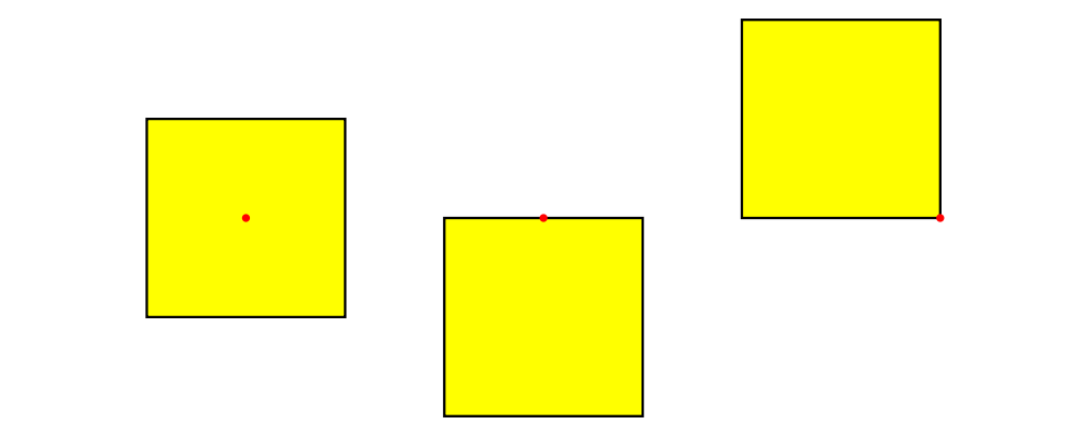
Functions like alignT (align Top) and alignBR (align Bottom Right) move the local origin to the edge of the envelope:

> s = square 1 # fc yellow
> example = hsep 0.5
>   [ s # showOrigin
>   , s # alignT  # showOrigin
>   , s # alignBR # showOrigin
>   ]

There are two things to note about the above example. First, notice how alignT and alignBR move the local origin of the square in the way you would expect. Second, notice that when placed "next to" each other using the (|||) operator (here implicitly via hsep), the squares are placed so that their local origins fall on a horizontal line.

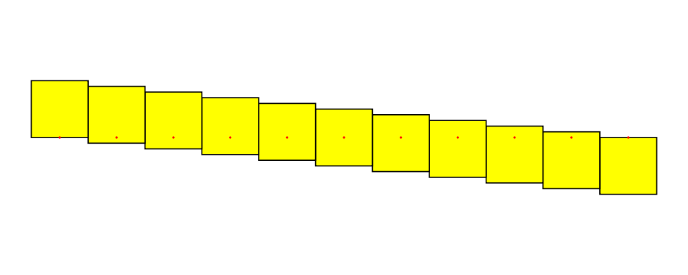
Functions like alignY allow finer control over the alignment. In the below example, the origin is moved to a series of locations interpolating between the bottom and top of the square:

> s = square 1 # fc yellow
> example = hcat . map showOrigin
>         $ zipWith alignY [-1, -0.8 .. 1] (repeat s)

To center an object along an axis we provide the functions centerX and centerY. An object can be simultaneously centered along both axes (actually along all of its basis vectors) using the center function (or centerXY in the specific case of two dimensions).

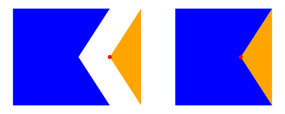
The align functions have sister functions like snugL and snugX that work the same way as alignL and alignX. The difference is that the snug class of functions use the trace as the boundary instead of the envelope. For example, here we want to snug a convex shape (the orange triangle) next to a concave shape (the blue polygon):

> import Diagrams.TwoD.Align
>
> concave = polygon ( with & polyType .~ PolyPolar [a, b, b, b]
>                   [ 0.25,1,1,1,1] & polyOrient .~ NoOrient )
>                   # fc blue # lw none
>   where
>     a = 1/8 @@ turn
>     b = 1/4 @@ turn
>
> convex = polygon (with & polyType .~ PolyPolar [a,b] [0.25, 1, 1]
>                        & polyOrient .~ NoOrient)
>                        # fc orange # lw none
>   where
>     a = 1/8 @@ turn
>     b = 3/4 @@ turn
>
> aligned = (concave # center # alignR # showOrigin)
>        <> (convex # center # alignL # showOrigin)
>
> snugged = (concave # center # snugR # showOrigin)
>        <> (convex # center # snugL # showOrigin)
>
> example = aligned ||| strutX 0.5 ||| snugged

The snugR function moves the origin of the blue polygon to the rightmost edge of its trace in the diagram on the right, whereas in the left diagram the alignR function puts it at the edge of the envelope.

Aligned composition

Sometimes, it is desirable to compose some diagrams according to a certain alignment, but without affecting their local origins. The composeAligned function can be used for this purpose. It takes as arguments an alignment function (such as alignT or snugL), a composition function of type [Diagram] -> Diagram, and produces a new composition function which works by first aligning the diagrams before composing them.

> example = (hsep 2 # composeAligned alignT) (map circle [5,1,3,2])
>         # showOrigin

3.5   Trails and paths

Trails and paths are some of the most fundamental tools in diagrams. They can be used not only directly to draw things, but also as guides to help create and position other diagrams.

For additional practice and a more "hands-on" experience learning about trails and paths, see the trails and paths tutorial.

Segments

The most basic component of trails and paths is a Segment, which is some sort of primitive path from one point to another. Segments are translationally invariant; that is, they have no inherent location, and applying a translation to a segment has no effect (however, other sorts of transformations, such as rotations and scales, have the effect you would expect). In other words, a segment is not a way to get from some particular point A to another point B; it is a way to get from wherever you currently happen to be to somewhere else.

Currently, diagrams supports two types of segment, defined in Diagrams.Segment:

  • A linear segment is simply a straight line, defined by an offset from its beginning point to its end point; you can construct one using straight.

  • A Bézier segment is a cubic curve defined by an offset from its beginning to its end, along with two control points; you can construct one using bezier3 (or bézier3, if you are feeling snobby). An example is shown below, with the endpoints shown in red and the control points in blue. Bézier curves always start off from the beginning point heading towards the first control point, and end up at the final point heading away from the last control point. That is, in any drawing of a Bézier curve like the one below, the curve will be tangent to the two dotted lines.

> illustrateBézier c1 c2 x2
>     =  endpt
>     <> endpt  # translate x2
>     <> ctrlpt # translate c1
>     <> ctrlpt # translate c2
>     <> l1
>     <> l2
>     <> fromSegments [bézier3 c1 c2 x2]
>   where
>     dashed  = dashingN [0.03,0.03] 0
>     endpt   = circle 0.05 # fc red  # lw none
>     ctrlpt  = circle 0.05 # fc blue # lw none
>     l1      = fromOffsets [c1] # dashed
>     l2      = fromOffsets [x2 ^-^ c2] # translate c2 # dashed
>
> x2      = r2 (3,-1) :: V2 Double     -- endpoint
> [c1,c2] = map r2 [(1,2), (3,0)]     -- control points
>
> example = illustrateBézier c1 c2 x2

Independently of the two types of segments explained above, segments can be either closed or open. A closed segment has a fixed endpoint relative to its start. An open segment, on the other hand, has an endpoint determined by its context; open segments are used to implement loops (explained in the Trails section below). Most users should have no need to work with open segments. (For that matter, most users will have no need to work directly with segments at all.)

If you look in the Diagrams.Segment module, you will see quite a bit of other stuff related to the implementation of trails (SegMeasure and so on); this is explained in more detail in the section Trail and path implementation details.

Functions from the Diagrams.TwoD.Curvature module can be used to compute the curvature of segments at various points. In future releases of diagrams this may be extended to tools for finding the curvature of trails and paths.

Trails

Trails are defined in Diagrams.Trail. Informally, you can think of trails as lists of segments laid end-to-end. Since segments are translation-invariant, so are trails. More formally, the semantics of a trail is a continuous (though not necessarily differentiable) function from the real interval \([0,1]\) to vectors in some vector space. This section serves as a reference on trails; for a more hands-on introduction, refer to the Trail and path tutorial.

There are two types of trail:

  • A loop, with a type like Trail' Loop v n, is a trail which forms a "closed loop", ending at the same place where it started.

    Loops in 2D can be filled, as in the example above.

  • A line, with a type like Trail' Line v n, is a trail which does not form a closed loop, that is, it starts in one place and ends in another.

    Actually, a line can in fact happen to end in the same place where it starts, but even so it is still not considered closed. Lines have no inside and outside, and are never filled.

    Lines are never filled, even when they happen to start and end in the same place!

Finally, the type Trail can contain either a line or a loop.

The most important thing to understand about lines, loops, and trails is how to convert between them.

  • To convert from a line or a loop to a trail, use wrapLine or wrapLoop (or wrapTrail, if you don't know or care whether the parameter is a line or loop).

  • To convert from a loop to a line, use cutLoop. This results in a line which just so happens to end where it starts.

  • To convert from a line to a loop, there are two choices:

    • closeLine adds a new linear segment from the end to the start of the line.

      > almostClosed :: Trail' Line V2 Double
      > almostClosed = fromOffsets $ (map r2
      >   [(2, -1), (-3, -0.5), (-2, 1), (1, 0.5)])
      >
      > example = pad 1.1 . center . fc orange . hsep 1
      >   $ [ almostClosed # strokeLine
      >     , almostClosed # closeLine # strokeLoop
      >     ]
    • glueLine simply modifies the endpoint of the final segment to be the start of the line. This is most often useful if you have a line which you know just so happens to end where it starts; calling closeLine in such a case would result in the addition of a gratuitous length-zero segment.

Lines form a monoid under concatenation. For example, below we create a two-segment line called spoke and then construct a starburst path by concatenating a number of rotated copies. Note how we call glueLine to turn the starburst into a closed loop, so that we can fill it (lines cannot be filled). strokeLoop turns a loop into a diagram, with the start of the loop at the local origin. (There are also analogous functions strokeLine and strokeTrail.)

> spoke :: Trail' Line V2 Double
> spoke = fromOffsets . map r2 $ [(1,3), (1,-3)]
>
> burst :: Trail' Loop V2 Double
> burst = glueLine . mconcat . take 13 . iterate (rotateBy (-1/13)) $ spoke
>
> example = strokeLoop burst # fc yellow # lw thick # lc orange

For convenience, there is also a monoid instance for Trail based on the instance for lines: any loops are first cut with cutLine, and the results concatenated. Typically this would be used in a situation where you know that all your trails actually contain lines.

Loops, on the other hand, have no monoid instance.

To construct a line, loop, or trail, you can use one of the following:

  • fromOffsets takes a list of vectors, and turns each one into a linear segment.

    > theLine = fromOffsets (iterateN 5 (rotateBy (1/20)) unitX)
    > example = theLine # strokeLine
    >         # lc blue # lw thick # center # pad 1.1
  • fromVertices takes a list of vertices, generating linear segments between them.

    > vertices = map p2 $ [(x,y) | x <- [0,0.2 .. 2], y <- [0,1]]
    > example = fromVertices vertices # strokeLine
    >         # lc red # center # pad 1.1
  • (~~) creates a simple linear trail between two points.

  • cubicSpline creates a smooth curve passing through a given list of points; it is described in more detail in the section on Splines.

    > vertices = map p2 . init $ [(x,y) | x <- [0,0.5 .. 2], y <- [0,0.2]]
    > theLine = cubicSpline False vertices
    > example = mconcat (iterateN 6 (rotateBy (-1/6)) theLine)
    >         # glueLine # strokeLoop
    >         # lc green # lw veryThick # fc aqua # center # pad 1.1
  • bspline creates a smooth curve controlled by a given list of points; it is also described in more detail in the section on Splines.

    > pts = map p2 (zip [0 .. 8] (cycle [0, 1]))
    > example = mconcat
    >   [ bspline pts
    >   , mconcat $ map (place (circle 0.1 # fc blue # lw none)) pts
    >   ]
  • fromSegments takes an explicit list of Segments, which can occasionally be useful if, say, you want to generate some Bézier curves and assemble them into a trail.

All the above functions construct loops by first constructing a line and then calling glueLine (see also the below section on TrailLike).

If you look at the types of these functions, you will note that they do not, in fact, return just Trails: they actually return any type which is an instance of TrailLike, which includes lines, loops, Trails, Paths (to be covered in an upcoming section), Diagrams, lists of points, and any of these wrapped in Located (see below). See the TrailLike section for more on the TrailLike class.

For details on other functions provided for manipulating trails, see the documentation for Diagrams.Trail. One other function worth mentioning is explodeTrail, which turns each segment in a trail into its own individual Path. This is useful when you want to construct a trail but then do different things with its individual segments. For example, we could construct the same starburst as above but color the edges individually:

> spoke :: Trail V2 Double
> spoke = fromOffsets . map r2 $ [(1,3), (1,-3)]
>
> burst = mconcat . take 13 . iterate (rotateBy (-1/13)) $ spoke
>
> colors = cycle [aqua, orange, deeppink, blueviolet, crimson, darkgreen]
>
> example = lw thick
>         . mconcat
>         . zipWith lc colors
>         . map strokeLocTrail . explodeTrail
>         $ burst `at` origin

(If we wanted to fill the starburst with yellow as before, we would have to separately draw another copy of the trail with a line width of zero and fill that; this is left as an exercise for the reader.)

Located

Something of type Located a consists, essentially, of a value of type a paired with a point. In this way, Located serves to transform translation-invariant things (such as Segments or Trails) into things with a fixed location. A Located Trail is a Trail where we have picked a concrete location for its starting point, and so on.

The module Diagrams.Located defines the Located type and utilities for working with it:

  • at is used to construct Located values, and is designed to be used infix, like someTrail `at` somePoint.

  • viewLoc, unLoc, and loc can be used to project out the components of a Located value.

  • mapLoc can be used to apply a function to the value of type a inside a value of type Located a. Note that Located is not a Functor, since it is not possible to change the contained type arbitrarily: mapLoc does not change the location, and the vector space associated to the type a must therefore remain the same.

Much of the utility of having a concrete type for the Located concept (rather than just passing around values paired with points) lies in the type class instances we can give to Located:

  • HasOrigin: translating a Located a simply translates the associated point, leaving the value of type a unaffected.

  • Transformable: only the linear component of transformations are applied to the wrapped value (whereas the entire transformation is applied to the location).

  • Enveloped: the envelope of a Located a is the envelope of the contained a, translated to the stored location (and similarly for Traced).

  • The TrailLike instance is also useful; see TrailLike.

Paths

A Path, also defined in Diagrams.Path, is a (possibly empty) collection of Located Trails. Paths of a single trail can be constructed using the same functions described in the previous section: fromSegments, fromOffsets, fromVertices, (~~), and cubicSpline, bspline.

Paths also form a Monoid, but the binary operation is superposition (just like that of diagrams). Paths with multiple components can be used, for example, to create shapes with holes:

> ring :: Path V2 Double
> ring = circle 3 <> (circle 2 # reversePath)
>
> example = ring # strokeP # fc purple

See the section on Fill rules for more information.

strokePath (alias strokeP) turns a path into a diagram, just as strokeTrail turns a trail into a diagram. (In fact, strokeTrail really works by first turning the trail into a path and then calling strokePath on the result.)

explodePath, similar to explodeTrail, turns the segments of a path into individual paths. Since a path is a collection of trails, each of which is a sequence of segments, explodePath actually returns a list of lists of paths.

For information on other path manipulation functions such as pathFromTrail, pathFromLocTrail, pathPoints, pathVertices, pathOffsets, scalePath, and reversePath, see the Haddock documentation in Diagrams.Path.

Vertices vs points

A vertex of a trail or path is defined as a sharp corner, i.e. a non-differentiable point. This is (mostly) independent of the implementation of trails and paths. A point, on the other hand, refers to the join point between two Segments, which is specific to the implementation of trails as collections of Segments.

For computing vertices, there are a number of functions like pathVertices, trailVertices, lineVertices, and loopVertices. Each of these also has a primed variant, like trailVertices', which takes an extra argument specifying a tolerance: in practice, where two segments join, we need some tolerance expressing how close the slopes of the segments must be in order to consider the join point differentiable (and hence not a vertex).

For computing points, there are variants pathPoints, trailPoints, linePoints, and loopPoints. However, these are (intentionally) not exported from Diagrams.Prelude. To use them, import Diagrams.Path or Diagrams.Trail.

In the example below, you can see that a circle has no vertices, whereas it has four points (exposing the implementation detail that a circle is constructed out of four Bézier segments; you should not rely on this!). On the other hand, a hexagon has the six vertices you would expect.

> import Diagrams.Trail  -- for trailPoints
>
> visPoints :: [P2 Double] -> Diagram B
> visPoints pts = atPoints pts (repeat (circle 0.05 # lw none # fc blue))
>
> example = hsep 0.5
>  [ circle 1 `beneath` visPoints (trailVertices (circle 1))
>  , circle 1 `beneath` visPoints (trailPoints (circle 1))
>  , hexagon 1 `beneath` visPoints (trailVertices (hexagon 1))
>  ]

Stroking trails and paths

The strokeTrail and strokePath functions, which turn trails and paths into diagrams respectively, have already been mentioned; they are defined in Diagrams.TwoD.Path. Both also have primed variants, strokeTrail' and strokePath', which take a record of StrokeOpts. Currently, StrokeOpts has two fields:

  • vertexNames takes a list of lists of names, and zips each list with a component of the path, creating point subdiagrams (using pointDiagram) associated with the names. This means that the names can be used to later refer to the locations of the path vertices (see Named subdiagrams). In the case of strokeTrail', only the first list is used.

    By default, vertexNames is an empty list.

  • queryFillRule specifies the fill rule (see Fill rules) used to determine which points are inside the diagram, for the purposes of its query (see Using queries). Note that it does not affect how the diagram is actually drawn; for that, use the fillRule function. (This is not exactly a feature, but for various technical reasons it is not at all obvious how to have this field actually affect both the query and the rendering of the diagram.)

    By default, queryFillRule is set to Winding.

There is also a method stroke, which takes as input any type which is an instance of ToPath, a type class with a single method:

> toPath :: (Metric (V t), OrderedField (N t))
>        => t -> Path (V t) (N t)

Calling stroke can sometimes produce errors complaining of an ambiguous type, which can happen if stroke is called on something which is itself polymorphic (e.g. because it can be any instance of TrailLike). The solution in this case is to use type-specific stroking functions like strokePath, strokeTrail, strokeLocLine, etc. See the ToPath reference for more information.

Offsets of segments, trails, and paths

Given a segment and an offset radius \(r\) we can make an offset segment that is the distance \(r\) from the original segment. More specifically, you can think of the offset as the curve traced by the end of a vector of length \(r\) perpendicular to the original curve. This vector goes on the right of the curve for a positive radius and on the left for a negative radius.

> import Diagrams.TwoD.Offset
>
> example :: Diagram B
> example = hsep 1 $ map f
>         [ straight p
>         , bézier3 (r2 (0,0.5)) (r2 (1,0.5)) p
>         ]
>   where
>     p = r2 (1,1)
>     f :: Segment Closed V2 Double -> Diagram B
>     f s =  fromSegments [s]
>         <> offsetSegment 0.1 0.2 s # strokeLocTrail # lc blue

Animate tracing an offset?

For a straight segment this will clearly be a parallel straight line with \(r\) as the distance between the lines. For an counter-clockwise arc of radius \(R\) the offset will be an arc with the same center, start and end angles, and radius \(r+R\). Cubic segments present a problem, however. The offset of a cubic Bézier curve could be a higher degree curve. To accommodate this we approximate the offset with a sequence of segments. We now have enough details to write the type for offsetSegment.

> offsetSegment :: Double -> Double -> Segment Closed V2 Double -> Located (Trail V2 Double)

The first parameter to offsetSegment is an epsilon factor \(\epsilon\). When the radius is multiplied by \(\epsilon\) we get the maximum allowed distance a point on the approximate offset can differ from the true offset. The final parameters are the radius and the segment. The result is a located trail. It is located because the offset's start will be distance \(r\) away from the segment start which is the origin.

If we can offset a segment we naturally will want to extend this to offset a trail. A first approach might be to simply map offsetSegment over the segments of a trail. But we quickly notice that if the trail has any sharp corners, the offset will be disconnected!

> import Diagrams.TwoD.Offset
>
> locatedTrailSegments t = zipWith at (trailSegments (unLoc t)) (trailVertices t)
>
> bindLoc f = join' . mapLoc f
>   where
>     join' x = let (p,a) = viewLoc x in translate (p .-. origin) a
>
> offsetTrailNaive :: Double -> Double -> Trail V2 Double -> Path V2 Double
> offsetTrailNaive e r = mconcat . map (pathFromLocTrail . bindLoc (offsetSegment e r))
>                      . locatedTrailSegments . (`at` origin)
>
> example :: Diagram B
> example = (p # strokeTrail <> offsetTrailNaive 0.1 0.3 p # stroke # lc blue)
>         # lw thick
>   where p = fromVertices . map p2 $ [(0,0), (1,0.3), (2,0), (2.2,0.3)]

First let's consider the outside corner where the adjacent offset segments do not cross. If we consider sweeping a perpendicular vector along the original trail we have a problem when we get to a corner. It is not clear what perpendicular means for that point. One solution is to take all points distance \(r\) from the corner point. This puts a circle around the corner of radius \(r\). Better is to just take the portion of that circle that transitions from what is perpendicular at the end of the first segment to what is perpendicular at the start of the next. We could also choose to join together offset segments in other sensible ways. For the choice of join we have the _offsetJoin field in the OffsetOpts record.

> import Diagrams.TwoD.Offset
>
> example :: Diagram B
> example = (p # strokeTrail <> o # strokeLocTrail # lc blue)
>         # lw thick
>   where
>     p = fromVertices . map p2 $ [(0,0), (1,0.3), (2,0), (2.2,0.3)]
>     o = offsetTrail' (with & offsetJoin .~ LineJoinRound) 0.3 p

Inside corners are handled in a way that is consistent with outside corners, but this yields a result that is most likely undesirable. Future versions of Diagrams will include the ability to clip inside corners with several options for how to do the clipping.

Update after implementing clipping.

There are other interesting ways we can join segments. We implement the standard line join styles and will also in the future provide the ability to specify a custom join.

> import Diagrams.TwoD.Offset
>
> example :: Diagram B
> example = hsep 0.5 $ map f [LineJoinMiter, LineJoinRound, LineJoinBevel]
>   where
>     f s = p # strokeTrail <> (offsetTrail' (with & offsetJoin .~ s) 0.3 p # strokeLocTrail # lc blue)
>     p = fromVertices . map p2 $ [(0,0), (1,0), (0.5,0.7)]

The LineJoinMiter style in particular can use more information to dictate how long a miter join can extend. A sharp corner can have a miter join that is an unbounded distance from the original corner. Usually, however, this long join is not desired. Diagrams follows the practice of most graphics software and provides a _offsetMiterLimit field in the OffsetOpts record. When the join would be beyond the miter limit, the join is instead done with a straight line as in the LineJoinBevel style. The OffsetOpts record then has three parameters:

> data OffsetOpts = OffsetOpts
>     { _offsetJoin       :: LineJoin
>     , _offsetMiterLimit :: Double
>     , _offsetEpsilon    :: Double
>     }

And the type for offsetTrail' is (offsetTrail simply uses the Default instance for OffsetOpts):

> offsetTrail  ::               Double -> Located (Trail V2 Double) -> Located (Trail V2 Double)
> offsetTrail' :: OffsetOpts -> Double -> Located (Trail V2 Double) -> Located (Trail V2 Double)
>
> offsetPath  ::               Double -> Path V2 Double -> Path V2 Double
> offsetPath' :: OffsetOpts -> Double -> Path V2 Double -> Path V2 Double

Notice this takes a Trail V2 Double which means it works for both Trail' Line V2 Double and Trail' Loop V2 Double. The second parameter is the radius for the offset. A negative radius gives a Line on the right of the curve, or a Loop inside a counter-clockwise Loop. For offsetPath we can simply map offsetTrail over the trails in the path in the most natural way.

Expand segments, trails, and paths

Expanding is just like the offset, but instead of producing a curve that follows one side we follow both sides and produce a Loop that can be filled representing all the area within a radius \(r\) of the original curve.

In addition to specifying how segments are joined, we now have to specify the transition from the offset on one side of a curve to the other side of a curve. This is given by the LineCap.

> data ExpandOpts = ExpandOpts
>     { _expandJoin       :: LineJoin
>     , _expandMiterLimit :: Double
>     , _expandCap        :: LineCap
>     , _expandEpsilon    :: Double
>     }
>
> expandTrail  ::               Double -> Located (Trail V2 Double) -> Path V2 Double
> expandTrail' :: ExpandOpts -> Double -> Located (Trail V2 Double) -> Path V2 Double
>
> expandPath  ::               Double -> Path V2 Double -> Path V2 Double
> expandPath' :: ExpandOpts -> Double -> Path V2 Double -> Path V2 Double

The functionality follows closely to the offset functions, but notice that the result of expandTrail is a Path V2 Double where offsetTrail resulted in a Located (Trail V2 Double). This is because an expanded Loop will be a pair of loops, one inside and one outside. To express this we need a Path.

> import Diagrams.TwoD.Offset
>
> example :: Diagram B
> example = (p # strokeTrail # lw veryThick # lc white <> e # strokePath # lw none # fc blue)
>   where
>     p = fromVertices . map p2 $ [(0,0), (1,0.3), (2,0), (2.2,0.3)]
>     e = expandTrail' opts 0.3 p
>     opts = with & expandJoin .~ LineJoinRound
>                 & expandCap  .~ LineCapRound

As long as the expanded path is filled with the winding fill rule we do not need to worry about having clipping for inside corners. It works out that the extra loop in the rounded line join will match with the outside corner. We currently implement all the LineCap styles, and plan to support custom styles in future releases.

> import Diagrams.TwoD.Offset
>
> example :: Diagram B
> example = hsep 0.5 $ map f [LineCapButt, LineCapRound, LineCapSquare]
>   where
>     f s =  p # strokeTrail # lw veryThick # lc white
>         <> expandTrail' (opts s) 0.3 p # stroke # lw none # fc blue
>     p = fromVertices . map p2 $ [(0,0), (1,0), (0.5,0.7)]
>     opts s = with & expandJoin .~ LineJoinRound
>                   & expandCap  .~ s

The TrailLike class

As you may have noticed by now, a large class of functions in the standard library—such as square, polygon, fromVertices, and so on—generate not just diagrams, but any type which is an instance of the TrailLike type class.

The TrailLike type class, defined in Diagrams.TrailLike, has only a single method, trailLike:

> trailLike :: Located (Trail (V t) (N t)) -> t

That is, a trail-like thing is anything which can be constructed from a Located Trail.

There are quite a few instances of TrailLike:

  • Trail: this instance simply throws away the location.

  • Trail' Line: throw away the location, and perform cutLoop if necessary. For example, circle 3 :: Trail' Line V2 Double is an open \(360^\circ\) circular arc.

  • Trail' Loop: throw away the location, and perform glueLine if necessary.

  • Path: construct a path with a single component.

  • Diagram b: as long as the backend b knows how to render paths, trailLike can construct a diagram by stroking the generated single-component path.

  • [Point v]: this instance generates the vertices of the trail.

  • Located (Trail v), of course, has an instance which amounts to the identity function. More generally, however, Located a is an instance of TrailLike for any type a which is also an instance. In particular, the resulting Located a has the location of the input Located Trail, and a value of type a generated by another call to trailLike. This is most useful for generating values of type Located (Trail' Line v) and Located (Trail' Loop v). For example, circle 3 # translateX 2 :: Located (Trail' Line V2 Double) is an open \(360^\circ\) circular arc centered at \((2,0)\).

It is quite convenient to be able to use, say, square 2 as a diagram, path, trail, list of vertices, etc., whichever suits one's needs. Otherwise, either a long list of functions would be needed for each primitive (like square, squarePath, squareTrail, squareVertices, squareLine, squareLocatedLine, ... ugh!), or else explicit conversion functions would have to be inserted when you wanted something other than what the square function gave you by default.

As an (admittedly contrived) example, the following diagram defines s as an alias for square 2 and then uses it at four different instances of TrailLike:

> s = square 2  -- a squarish thingy.
>
> blueSquares = atPoints  (concat . pathVertices $ s) {- 1 -}
>                 (replicate 4 (s {- 2 -} # scale 0.5) # fc blue)
> paths       = lc purple . stroke $ star (StarSkip 2) s {- 3 -}
> aster       = center . lc green . strokeLine
>             . mconcat . take 5 . iterate (rotateBy (1/5))
>             . onLineSegments init
>             $ s {- 4 -}
> example = (blueSquares <> aster <> paths)

Exercise: figure out which occurrence of s has which type. (Answers below.)

At its best, this type-directed behavior results in a "it just works/do what I mean" experience. However, it can occasionally be confusing, and care is needed. The biggest gotcha occurs when combining a number of shapes using (<>) or mconcat: diagrams, paths, trails, and lists of vertices all have Monoid instances, but they are all different, so the combination of shapes has different semantics depending on which type is inferred.

> ts = mconcat . iterateN 3 (rotateBy (1/9)) $ triangle 1
> example = (ts ||| strokeP ts ||| strokeLine ts ||| fromVertices ts) # fc red

The above example defines ts by generating three equilateral triangles offset by 1/9 rotations, then combining them with mconcat. The sneaky thing about this is that ts can have the type of any TrailLike instance, and it has completely different meanings depending on which type is chosen. The example uses ts at each of four different monoidal TrailLike types:

  • Since example is a diagram, the first ts, used by itself, is also a diagram; hence it is interpreted as three equilateral triangle diagrams superimposed on one another with atop.

  • strokeP turns Paths into diagrams, so the second ts has type Path V2 Double. Hence it is interpreted as three closed triangular paths superimposed into one three-component path, which is then stroked.

  • strokeLine turns Trail' Lines into diagrams, so the third occurrence of ts has type Trail' Line V2 Double. It is thus interpreted as three open triangular trails sequenced end-to-end into one long open trail. As a line (i.e. an open trail), it is not filled (in order to make it filled we could replace strokeLine ts with strokeLoop (glueLine ts)).

  • The last occurrence of ts is a list of points, namely, the concatenation of the vertices of the three triangles. Turning this into a diagram with fromVertices generates a single-component, open trail that visits each of the points in turn.

Of course, one way to avoid all this would be to give ts a specific type signature, if you know which type you would like it to be. Then using it at a different type will result in a type error, rather than confusing semantics.

Answers to the square 2 type inference challenge:

  1. Path V2 Double

  2. Diagram b V2 Double

  3. [Point V2 n]

  4. Trail' Line V2 Double

Segments and trails as parametric objects

Both segments and trails, semantically, can be seen as parametric functions: that is, for each value of a parameter within some given range (usually \([0,1]\)), there is a corresponding vector value (or point, for Located segments and trails). The entire collection of such vectors or points makes up the segment or trail.

The Diagrams.Parametric module provides tools for working with segments and trails as parametric functions.

Parametric

As explained above, parametric objects can be viewed semantically as functions. In particular, parametric objects of type p can be seen as functions of type Scalar (V p) -> Codomain p, where the type family Codomain is defined in such a way as to make this true. For example, Codomain (Trail V2 Double) ~ V2 Double, because a trail can be thought of as a function Double -> V2 Double.

The Parametric class defines the single method atParam which yields this parametric view of an object:

> atParam :: Parametric p => p -> Scalar (V p) -> Codomain p

(Note that it is not possible to convert in the other direction—every function of type Scalar (V p) -> Codomain p need not correspond to something of type p. For example, to convert from a function to a trail one would need at the very least a guarantee of continuity; segments are even more restricted.)

> spline :: Located (Trail V2 Double)
> spline = cubicSpline False [origin, 0 ^& 1, 1 ^& 1, 1 ^& 0] # scale 3
> pts = map (spline `atParam`) [0, 0.1 .. 1]
> spot = circle 0.2 # fc blue
>
> example = mconcat (map (place spot) pts) <> strokeLocTrail spline

Instances of Parametric include:

  • Segment Closed: The codomain is the type of vectors. Note there is no instance for Segment Open, since additional context is needed to determine the endpoint, and hence the parametrization, of an open segment.

  • FixedSegment: The codomain is the type of points.

  • Trail': The codomain is the vector space. Note that there is no difference between Line and Loop.

  • Trail: same as the instance for Trail'.

  • Located a: as long as a is also Parametric and the codomain of a is a vector space, Located a is parametric with points as the codomain. For example, calling atParam on a Located (Trail V2 Double) returns a P2 Double.

Paths are not Parametric, since they may have multiple trail components and there is no canonical way to assign them a parametrization.

DomainBounds

The domainLower and domainUpper functions simply return the lower and upper bounds for the parameter. By default, these will be \(0\) and \(1\), respectively. However, it is possible to have objects parameterized over some interval other than \([0,1]\).

EndValues

The EndValues class provides the functions atStart and atEnd, which return the value at the start and end of the parameter interval, respectively. In other words, semantically we have atStart x = x `atParam` domainLower x, but certain types may have more efficient or accurate ways of computing their start and end values (for example, Bézier segments explicitly store their endpoints, so there is no need to evaluate the generic parametric form).

Sectionable

The Sectionable class abstracts over parametric things which can be split into multiple sections (for example, a trail can be split into two trails laid end-to-end). It provides three methods:

  • splitAtParam :: p -> Scalar (V p) -> (p, p) splits something of type p at the given parameter into two things of type p. The resulting values will be linearly reparameterized to cover the same parameter space as the parent value. For example, a segment with parameter values in \([0,1]\) will be split into two shorter segments which are also parameterized over \([0,1]\).

  • section :: p -> Scalar (V p) -> Scalar (V p) -> p extracts the subpart of the original lying between the given parameters, linearly reparameterized to the same domain as the original.

  • reverseDomain :: p -> p reverses the parameterization. It probably should not be in this class and is likely to move elsewhere in future versions.

HasArcLength

HasArcLength abstracts over parametric things with a notion of arc length. It provides five methods:

  • arcLengthBounded approximates the arc length of an object to within a given tolerance, returning an interval which is guaranteed to contain the true arc length.

  • arcLength is similar to arcLengthBounded, but returns a single length value instead of an interval.

  • stdArcLength approximates the arc length up to a standard accuracy of \(\pm 10^{-6}\).

  • arcLengthToParam converts an arc length to a parameter, up to a given tolernace

  • stdArcLengthToParam is like arcLengthToParam, but using a standard accuracy of \(\pm 10^{-6}\).

Adjusting length

Anything which is an instance of DomainBounds, Sectionable, and HasArcLength can be "adjusted" using the adjust function, which provides a number of options for changing the length and extent.

Computing tangents and normals

The Diagrams.Tangent module contains functions for computing tangent vectors and normal vectors to segments and trails, at an arbitrary parametmer (tangentAtParam, normalAtParam) or at the start or end (tangentAtStart, tangentAtEnd, normalAtStart, normalAtEnd). (The start/end functions are provided because such tangent and normal vectors may often be computed more quickly and precisely than using the general formula with a parameter of 0 or 1.)

Splines

Constructing Bézier segments by hand is tedious. The Diagrams.CubicSpline module provides two functions for creating smooth curves given a list of points.

The cubicSpline function, given a list of points, constructs a smooth curved path passing through each point in turn. The first argument to cubicSpline is a boolean value indicating whether the path should be closed.

> pts = map p2 [(0,0), (2,3), (5,-2), (-4,1), (0,3)]
> spot = circle 0.2 # fc blue # lw none
> mkPath closed = position (zip pts (repeat spot))
>              <> cubicSpline closed pts
> example = mkPath False ||| strutX 2 ||| mkPath True

For more precise control over the generation of curved paths, see the Diagrams.TwoD.Path.Metafont module from diagrams-contrib, which also has its own tutorial.

Diagrams.CubicSpline also provides the bspline function, which creates a smooth curve (to be precise, a uniform cubic B-spline) with the given points as control points. The curve begins and ends at the first and last points, but in general does not pass through the intermediate points.

> pts = map p2 (zip [0 .. 8] (cycle [0, 1]))
> example = mconcat
>   [ bspline pts
>   , mconcat $ map (place (circle 0.1 # fc blue # lw none)) pts
>   ]

One major difference between cubicSpline and bspline is that the curves generated by cubicSpline depend on the control points in a global way—that is, changing one control point could alter the entire curve—whereas with bspline, each control point only affects a local portion of the curve.

Fill rules

There are two main algorithms or "rules" used when determining which areas to fill with color when filling the interior of a path: the winding rule and the even-odd rule. The rule used to draw a path-based diagram can be set with fillRule, defined in Diagrams.TwoD.Path. For simple, non-self-intersecting paths, determining which points are inside is quite simple, and the two algorithms give the same results. However, for self-intersecting paths, they usually result in different regions being filled.

> loopyStar = fc red
>           . mconcat . map (cubicSpline True)
>           . pathVertices
>           . star (StarSkip 3)
>           $ regPoly 7 1
> example = loopyStar # fillRule EvenOdd
>       ||| strutX 1
>       ||| loopyStar # fillRule Winding
  • The even-odd rule specifies that a point is inside the path if a straight line extended from the point off to infinity (in one direction only) crosses the path an odd number of times. Points with an even number of crossings are outside the path. This rule is simple to implement and works perfectly well for non-self-intersecting paths. For self-intersecting paths, however, it results in a pattern of alternating filled and unfilled regions, as seen in the above example. Sometimes this pattern is desirable for its own sake.

  • The winding rule specifies that a point is inside the path if its winding number is nonzero. The winding number measures how many times the path "winds" around the point, and can be intuitively computed as follows: imagine yourself standing at the given point, facing some point on the path. You hold one end of an (infinitely stretchy) rope; the other end of the rope is attached to a train sitting at the point on the path at which you are looking. Now the train begins traveling around the path. As it goes, you keep hold of your end of the rope while standing fixed in place, not turning at all. After the train has completed one circuit around the path, look at the rope: if it is wrapped around you some number of times, you are inside the path; if it is not wrapped around you, you are outside the path. More generally, we say that the number of times the rope is wrapped around you (positive for one direction and negative for the other) is the point's winding number.

    Draw a picture of you and the train

    For example, if you stand outside a circle looking at a train traveling around it, the rope will move from side to side as the train goes around the circle, but ultimately will return to exactly the state in which it started. If you are standing inside the circle, however, the rope will end up wrapped around you once.

    For paths with multiple components, the winding number is simply the sum of the winding numbers for the individual components. This means, for example, that "holes" can be created in shapes using a path component traveling in the opposite direction from the outer path.

    This rule does a much better job with self-intersecting paths, and it turns out to be (with some clever optimizations) not much more difficult to implement or inefficient than the even-odd rule.

You should be aware that queries (see Using queries) use the winding rule by default, and are not affected by the path fill rule attribute. Thus, if you apply the even-odd rule to a diagram, the query may not match in the way you expect. For this reason, if you want to make a shape with holes in it, it is usually better to form the holes from paths winding in the opposite direction (using reversePath and the winding rule) than from the even-odd rule. For example, in the diagram below, the annulus on the left is formed using the even-odd fill rule, and the one on the right with the default winding rule and a reversed inner circle. The dark blue points indicate places where the associated query evaluates to true.

> points = [x ^& 0 | x <- [-2.3, -2.1 .. 2.3]]
> dia1 = (circle 2 <> circle 1) # strokeP # fillRule EvenOdd # rotateBy (1/100)
> dia2 = (circle 2 <> reversePath (circle 1)) # strokeP # rotateBy (1/100)
>
> illustrate d = ((d # fc grey) `beneath`) . mconcat . map drawPt $ points
>   where
>     drawPt p | inquire d p = circle 0.1 # fc blue # moveTo p
>              | otherwise   = circle 0.07 # fc lightblue # moveTo p
>
> example = illustrate dia1 ||| strutX 1 ||| illustrate dia2

If you do want to make a diagram whose query uses the even-odd rule, you can use the strokePath' function.

Clipping

With backends that support clipping, paths can be used to clip other diagrams. Only the portion of a clipped diagram falling inside the clipping path will be drawn.

> example = square 3
>         # fc green
>         # lw veryThick
>         # clipBy (square 3.2 # rotateBy (1/10))

Several functions are available, depending on what envelope and trace you want the resulting diagram to have. clipBy uses the envelope and trace of the original diagram. clipped uses the envelope and trace of the clipping path. clipTo uses the intersection of the two envelopes, and a trace which matches the displayed outline of the diagram. Note that in general the intersection of envelopes is larger than the envelope of an intersection. Diagrams does not have a function which returns the tight envelope of the intersection.

Altering a diagram's envelope can also be accomplished using withEnvelope (see Envelope-related functions). The rectEnvelope function is also provided for the special case of setting a diagram's envelope to some rectangle, often used for the purpose of selecting only a part of a diagram to be "viewed" in the final output. It takes a point—the lower-left corner of the viewing rectangle—and the vector from the lower-left to upper-right corner.

> circles = (c ||| c) === (c ||| c) where c = circle 1 # fc fuchsia
> example = circles # center # rectEnvelope (p2 (-1,-1)) (r2 (1.3, 0.7))

Note in the above example how the actual portion of the diagram that ends up being visible is larger than the specification given to rectEnvelope—this is because the aspect ratio of the requested output image does not match the aspect ratio of the rectangle given to rectEnvelope (and also because of the use of frame by the framework which renders the user manual examples). If the aspect ratios matched the viewed portion would be exactly that specified in the call to rectEnvelope.

Boolean operations on paths

The Diagrams.TwoD.Path.Boolean module from diagrams-contrib contains functions for computing boolean combinations of paths, such as union, intersection, difference, and symmetric difference.

> import qualified Diagrams.TwoD.Path.Boolean as B
>
> thing1, thing2 :: Path V2 Double
> thing1 = square 1
> thing2 = circle 0.5 # translate (0.5 ^& (-0.5))
>
> example = hsep 0.5 . fc green . map strokePath $
>   [ B.union        Winding (thing1 <> thing2)
>   , B.intersection Winding thing1     thing2
>   , B.difference   Winding thing1     thing2
>   , B.exclusion    Winding thing1     thing2
>   ]

Trail and path implementation details

Trails are implemented using finger trees: in particular, lines are finger trees of closed segments, while loops consist of a finger tree of closed segments plus a single final open segment.

The benefit of using a finger tree (instead of just, say, a list, or even a Seq structure from Data.Sequence) is that it allows caching monoidal "measures" of the entire trail. In particular, the finger trees underlying trails cache

  • the number of segments

  • the total arc length (up to a standard error tolerance)

  • the total offset (vector from start to end)

  • the envelope

For more details, see the Diagrams.Segment and Diagrams.Trail modules.

Another interesting aspect of the implementation is that upon stroking a path to form a diagram, instead of simply putting the entire path into a primitive, we separate out the lines and loops into two path primitives. This is helpful for backends because they often have to do some active work to avoid filling lines, and if diagrams-lib did not do this separation, they would essentially have to end up doing it themselves.

3.6   Arrows

Diagrams.TwoD.Arrow and Diagrams.TwoD.Arrowheads provide specialized functionality for drawing arrows. Note that arrows are drawn with scale-invariant heads and tails (see Scale-invariance). Arrows can be used to connect various things including literal points, named subdiagrams, or their traces. For more detailed information, examples, and exercises, see the Arrows tutorial.

To create arrows, one may use the functions:

  • arrowBetween to connect points;

  • connect to connect diagrams;

  • connectOutside to connect points on the boundary (trace) of diagrams (for an example, see the symmetry cube example in the gallery);

  • connectPerim to connect points on the traces of diagrams at particular external angles;

  • arrowAt to place an arrow at a point;

  • arrowV to create an arrow with the magnitude and direction of a given vector.

> sPt = 0.50 ^& 0.50
> ePt = 5.2 ^& 0.50
>
> -- Connect two points.
> ex1 = arrowBetween sPt ePt
>
> d = octagon 1 # lc blue # lw ultraThick # showOrigin
> ds = d # named "1" ||| strut 3 ||| d # named "2"
>
> -- Connect two diagrams and two points on their trails.
> ex23 = ds # connect "1" "2"
>           # connectPerim "1" "2" (15/16 @@ turn) (9/16 @@ turn)
>
> -- Place an arrow at (0,0) the size and direction of (0,1).
> ex4 = arrowAt (0 ^& 0) unit_Y
>
> example = (ex1
>           ===
>           strutY 0.5
>           ===
>           (ex23 <> ex4)) # center

Notice that the arrows in the above diagram all have the same dart shaped head, no tail, and a straight shaft. All of these aspects, and many others, can be customized using companion functions to the ones above, whose names end with an apostrophe. For example, the companion to connect is connect'. These companion functions take an extra ArrowOpts record, whose fields are:

  • arrowHead and arrowTail, to specify the shape of the head and tail. The Diagrams.TwoD.Arrowheads module exports the arrowheads tri, dart, spike, thorn, lineHead, and noHead; the default is dart. For tails we have quill, block, lineTail, and noTail; noTail is the default. Additionally, any head can be used as a tail by appending a ' (e.g. dart'). There are also functions that can be used to create custom heads and tails (see Diagrams.TwoD.Arrow).

  • arrowShaft is any Trail V2 Double; it will be sized automatically to fit between the endpoints of the arrow.

  • headLength and tailLength specify the size of the head and tail, defined as the length of the head or tail plus the joint connecting it to the shaft. Their value is of type Measure V2 Double (see Measurement units). The default value is normal which is a synonym for normalized 0.035. A traversal called lengths sets both the headLength and tailLength at the same time.

  • headGap and tailGap both default to none and are used to indicate the amount of space between the end of the arrow and the location it is pointing at. They are also of type Measure V2 Double. A traversal called gaps is provided to set both the headGap and tailGap simultaneously.

  • headStyle, tailStyle and shaftStyle are used to pass in style functions like fc blue . opacity 0.75 to customize parts of the arrow. (By default, the entire arrow, including head and tail, is drawn using the current line texture.)

The Lenses headTexture, tailTexture, and shaftTexture are provided for conveniently setting the texture of a head or tail. Additionally, the function solid converts a color to a texture. For example, (with & headTexture .~ solid blue) will set the head color to blue.

The following example demonstrates the use of various ArrowOpts. See Named subdiagrams for the use of names and the named function.

> c = circle 2 # fc lightgray # lw none # showOrigin
>
> row1 = hsep 3
>   [ c # named "1", c # named "3"
>   , c # named "5", c # named "7"
>   ]
> row2 = hsep 3
>   [ c # named "2", c # named "4"
>   , c # named "6", c # named "8"
>   ]
>
> d = row1 === strutY 5 === row2
>
> shaft1 = trailFromVertices (map p2 [(0, 0), (1, 0), (1, 0.2), (2, 0.2)])
> shaft2 = cubicSpline False (map p2 [(0, 0), (1, 0), (1, 0.2), (2, 0.2)])
> shaft3 = arc xDir (1/6 @@ turn)
>
> example = d
>    # connect' (with & arrowTail .~ quill & lengths .~ large
>                     & tailTexture .~ solid orange & headTexture .~ solid orange
>                     & arrowHead .~ spike
>                     & shaftStyle %~ lw veryThick ) "1" "2"
>    # connect' (with & arrowTail .~ thorn' & lengths .~ large
>                     & arrowHead .~ thorn
>                     & arrowShaft .~ shaft1 & shaftStyle %~ lw veryThick ) "3" "4"
>    # connect' (with & arrowTail .~ block & gaps .~ small
>                     & arrowHead .~ dart & headLength .~ large
>                     & arrowShaft .~ shaft2
>                     & headStyle %~ fc blue & tailStyle %~ fc blue
>                     & shaftStyle %~ lw veryThick . lc blue ) "5" "6"
>    # connect' (with & arrowShaft .~ shaft3
>                     & arrowHead .~ tri & headLength .~ large
>                     & headStyle %~ fc red . opacity 0.5
>                     & shaftStyle %~ lw veryThick . lc black . opacity 0.5 ) "7" "8"

3.7   Text

Note: The various backends differ substantially in their text-handling capabilities. For this and other reasons, there are two ways to add text to diagrams, each with advantages. The method in this section is heavily dependent on backend support. The Cairo backend has the most complete support; in particular, this is the best approach for complex (non-Roman) scripts. The Rasterific backend also has good text support, via the FontyFruity package. You may also want to look at the SVGFonts package, described in the section Native font support below, which converts text directly into Paths.

Text objects, defined in Diagrams.TwoD.Text, can be created most simply with the text function, which turns a String into a diagram with (centered) text:

> example = text "Hello world!" <> rect 8 1

Text with different alignments can be created using topLeftText or baselineText (or, more generally, alignedText, though it is not supported by all backends—the SVG backend in particular only supports an approximation to alignedText):

> pt = circle 0.1 # fc red
>
> t1 = pt <> topLeftText         "top left"   <> rect 8 1
> t2 = pt <> baselineText        "baseline"   <> rect 8 1
> t3 = pt <> alignedText 0.7 0.5 "(0.7, 0.5)" <> rect 8 1
>
> d1 =/= d2 = d1 === strutY 2 === d2
> example = t1 =/= t2 =/= t3

The most important thing to keep in mind when working with text objects is that they take up no space: they have a point envelope at the origin, i.e. for the purposes of things like beside, they have a width and height of zero. (Note, however, this is not the same as having an empty envelope. In particular, they still behave in an intuitive manner when included as arguments to things like hcat.) If we omitted the rectangle from the above example, there would be no output. Except: the PGF backend has the ability to create enveloped text as does the Rasterific backend by using the Diagrams.Backend.Rasterific.Text module.

Text objects take up no space!

The main reason for this is that computing the size of some text in a given font is rather complicated, and diagrams cannot (yet) do it natively.

Text is colored with the current fill color (see Color and Opacity). Various other attributes of text can be set using font, fontWeight, and fontSlant. The convenience function italic and oblique are provided for setting the font slant, and for weight there are functions bold, bolder, lighter, thinWeight, ultraLight, light, mediumWeight, heavy, semiBold, and ultraBold. Note that many backends do not support font weights besides bold; the SVG backend supports all font weights.

> text' s t = text t # fontSize (local s) <> strutY (s * 1.3)
> example = center $
>       text' 10 "Hello" # italic
>   === text' 5 "there"  # bold # font "freeserif"
>   === text' 3 "world"  # fc green

Font size

Font size is set using the fontSize function, and is specified by a value of type Measure V2 Double (see Measurement units).

  • Text with a local font size is measured relative to its local vector space. Such text is transformed normally by any transformations applied to it. For example, in the diagram below, fontSize (local 1) is specified (this is actually the default, so it could be omitted without changing the diagram). Note how the F's are the same size as a unit box, and scale, stretch, and rotate along with it.

    > eff = (text "F" <> square 1) # fontSize (local 1)
    >
    > example = hcat
    >   [eff, eff # scale 2, eff # scaleX 2, eff # scaleY 2, eff # rotateBy (1/12)]
  • Text whose font size is specified in any measurement other than local (that is, normalized, global, or output) behaves differently.

    > eff = (text "F" <> square 1) # fontSize (normalized 0.1)
    >
    > example = hcat
    >   [eff, eff # scale 2, eff # scaleX 2, eff # scaleY 2, eff # rotateBy (1/12)]

    There are several things to notice about the above example diagram, which is identical to the previous one except for the fact that normalized 0.1 is used instead of local 1:

    • The F's are 1/10th the size of the overall diagram. If we added more copies of eff to the right, but kept the physical size of the rendered image the same, the F's would remain the same physical size on the screen, but would get bigger relative to the boxes (since the boxes would be smaller in absolute terms).

    • The F's are all about the same size—in particular, the uniform scaling applied to the second F has no effect, and the fourth F is not twice as tall as the others. Note, however, that the final F rotates with the square as expected. Note also that the third and fourth F's are squished, as one would expect from a non-uniform scaling. The hand-wavy slogan is that non-local-sized text is "affected by transformations, but without changing size".

      The technical specification is that applying a transformation \(T\) to non-local-sized text actually results in applying the transformation \(\frac{1}{|T|} T\), where \(|T|\) denotes the average scaling factor of the transformation \(T\), computed as the square root of the positive determinant of \(T\). This behaves nicely: for example, the average scaling factor of scale k is k, so applying a uniform scaling to non-local-sized text has no effect; it is also compositional, so applying t and then s to some text has exactly the same effect as applying s <> t. For more information, see the avgScale function and the comments associated with its source code.

Native font support

The SVGFonts package implements native text support for diagrams, using fonts in the SVG format (note that it can be used with any backend, not just the SVG backend). Among other things, it provides its own svgText function which can be used to convert text into a path tracing the outline of the text. Here is a simple example:

> import qualified Graphics.SVGFonts as SF
>
> text' font h s
>   = s
>   # SF.svgText def { SF.textFont = font }
>   # SF.fit_height h
>   # SF.set_envelope
>   # lw none
>
> example = do
>   font <- lin2
>   return $ text' font 5 "Hello" # fc blue ||| text' font 3 "world" # fc green

For more details and examples, see the Haddock documentation. Note that the API of the SVGFonts package changed quite a bit in version 1.8. For help porting your existing SVGFonts code to version 1.8, see the SVGFonts README.

3.8   Images

The Diagrams.TwoD.Image module provides basic support for including both external and embedded images in diagrams. Support for images varies by backend. Only the cairo backend supports external images. The rasterific backend supports embedded images of many formats and the SVG backend supports embedded PNG images.

To create an embedded diagram from an image file call loadImageEmb to read the image from a file path using JuicyPixels and return a DImage Embedded. Then use image to convert the DImage Embedded to a diagram. You can also create a diagram with an embedded image by supplying a function that maps pixel coordinates to AlphaColours plus a width and a height to the rasterDia function. For example, the below code uses rasterDia to visualize the multiplication table for the group \(U_7\) of natural numbers \(\{0, \dots, 6\}\) under multiplication mod 7.

> import Data.Colour.Palette.BrewerSet
>
> no = (circle 1 <> hrule 2 # rotateBy (1/8))
>    # lwO 40 # lc red # frame 0.2
> noPhoneIO = do
>   res <- loadImageEmb "doc/static/phone.png"
>   return $ case res of
>     Left err    -> mempty
>     Right phone -> no <> image phone # sized (dims2D 1.5 1.5)
>
> colors = brewerSet YlGn 7
> u7 = rasterDia
>   (\x y -> opaque (colors !! ((x `div` 100) * (y `div` 100) `mod` 7)))
>   700 700
>   # sized (dims2D 2 2)
>
> example = do
>   noPhone <- noPhoneIO
>   return $ noPhone ||| strutX 1.5 ||| u7

The function loadImageExt checks to make sure the file exists, uses JuicyPixels to determine its size and returns a reference to the image. On the other hand uncheckedImageRef simply packages the reference with a width and height to make a DImage External, without checking to make sure the image exists.

When using loadImageEmb and loadImageExt you do not need to provide the width and height of the image, as they will be calculated by JuicyPixels. Otherwise you must specify both a width and a height for each image. In this case you might hope to be able to specify just a width or just a height, and have the other dimension computed so as to preserve the image's aspect ratio. However, there is no way for diagrams to query an image's aspect ratio until rendering time, but (until such time as a constraint solver is added) it needs to know the size of the image when composing it with other subdiagrams. Hence, both dimensions must be specified, and for the purposes of positioning relative to other diagrams, the image will be assumed to occupy a rectangle of the given dimensions.

However, note that the image's aspect ratio will be preserved: if you specify dimensions that do not match the actual aspect ratio of the image, blank space will be left in one of the two dimensions to compensate. If you wish to alter an image's aspect ratio, you can do so by scaling nonuniformly with scaleX, scaleY, or something similar.

Current backend support for images can be summarized as follows:

  • Cairo: external PNG

  • SVG: embedded PNG; also PNG and JPG via a "native" extension (see below)

  • Rasterific: embedded PNG, JPG, TIF, BMP and GIF.

  • PGF: external PDF, JPG and PNG; embedded ImageRGB8.

Besides Embedded and External images, there is a third Native type which supports image formats particular to a specific backend. For more information, see "Diagrams.TwoD.Image":mod: as well as the documentation for individual backends.

4   Advanced tools for diagram creation

This section covers some of the more advanced tools provided by the core and standard libraries for constructing diagrams. Most of the content in this section is applicable to diagrams in any vector space, although 2D diagrams are used as illustrations.

4.1   Envelopes

The Envelope type, defined in Diagrams.Core.Envelope, encapsulates envelopes (see envelopes and local vector spaces). Things which have an associated envelope—including diagrams, segments, trails, and paths—are instances of the Enveloped type class.

Envelopes are used implicitly when placing diagrams next to each other (see Juxtaposing diagrams) or when aligning diagrams (see Alignment).

The Enveloped class

All objects with an associated envelope are instances of the Enveloped type class. This includes diagrams, segments, trails, and paths. Enveloped provides a single method,

> getEnvelope :: Enveloped a => a -> Envelope (V a) (N a)

which returns the envelope of an object.

In addition, the list type [b] is an instance of Enveloped whenever b is. The envelope for a list is simply the combination of all the individual envelopes of the list's elements—that is, an envelope that contains all of the list elements. In conjunction with the Transformable instance for lists (see The Transformable class), this can be used to do things such as apply an alignment to a list of diagrams considered as a group. For some examples and an explanation of why this might be useful, see Delayed composition.

4.2   Traces

Envelopes are useful for placing diagrams relative to one another, but they are not particularly useful for finding actual points on the boundary of a diagram. Finding points on the boundary of a diagram can be useful for things like drawing lines or arrows between two shapes, or deciding how to position another diagram relative to a given one.

Every diagram (and, more generally, anything which is an instance of the Traced type class) has a trace, a function which is like an "embedded ray tracer" for finding points on the diagram boundary. In particular, the trace function takes a ray as input (represented by a pair (p,v) of a base point and a vector) and returns a sorted list of parameters t such that p .+^ (t *^ v) is a point of intersection between the ray and the boundary of the diagram.

Normally, a trace is accessed using one of the four functions rayTraceV, rayTraceP, maxRayTraceV, and maxRayTraceP.

  • rayTraceV takes as inputs a base point p, a vector v, and any instance of Traced. It looks for intersection points with the given object along the ray determined by p and v, and finds the smallest positive scalar t such that p .+^ (t *^ v) is a point of intersection between the ray and the boundary of the Traced object. If such a t exists, it returns the vector from p to the intersection point, that is, t *^ v. If there is no such intersection, rayTraceV returns Nothing.

    Intuitively, restricting to positive t-values means that only intersection points "in front of" the point p (that is, in the direction of v) are considered. This tends to be the most intuitive behavior, and parallels the way raytracers work—think of p as the location of the "camera" and v as the direction the camera is pointing. If you want to consider negative t-values, see the traceV family of functions, described below, or use getTrace to access the list of all intersection parameters directly.

    > import Data.Maybe (fromMaybe)
    >
    > drawV v = arrowAt origin v
    >
    > drawTraceV v d
    >   = lc green $
    >     fromMaybe mempty
    >       ((origin ~~) <$> rayTraceP origin v d)
    > illustrateTraceV v d = (d <> drawV v <> drawTraceV v d) # showOrigin
    >
    > example = hsep 1
    >         . map (illustrateTraceV (0.5 *^ (r2 (1, 1))))
    >         $ [ circle 1 # translate (r2 (-1.5, -1.5))
    >           , circle 1
    >           , circle 1 # translate (r2 (1.5, 1.5))
    >           ]
  • rayTraceP works similarly, except that it returns the point of intersection itself, which lies on the boundary of the object, or Nothing if there is no such point.

    That is, rayTraceP p v x == Just p' if and only if rayTraceV p v x == Just (p' .-. p).

    The below diagram illustrates the use of the rayTraceP function to identify points on the boundaries of several diagrams.

    > {-# LANGUAGE TypeFamilies #-}
    >
    > import Data.Maybe (mapMaybe)
    > illustrateTrace :: (TrailLike a, Traced a, Semigroup a, Monoid a, V a ~ V2) => a -> a
    > illustrateTrace d = d <> traceLines
    >   where
    >     traceLines  = mconcat
    >                 . mapMaybe traceLine
    >                 . iterateN 30 (rotateBy (1/60))
    >                 $ unitX
    >     traceLine v = (basePt ~~) <$> traceP basePt v d
    >     basePt = p2 (0, -2)
    >
    > example
    >   = hsep 1
    >   . map illustrateTrace
    >   $ [ square 1
    >     , circle 1
    >     , triangle 1 # rotateBy (-1/4) ||| triangle 1 # rotateBy (1/4)
    >     ]
  • maxRayTraceV and maxRayTraceP are similar to rayTraceV and rayTraceP, respectively, except that they look for the largest positive t-value, that is, the furthest intersection point in the direction of v. Again, intersection points in the opposite direction from v are not considered.

  • The traceV, traceP, maxTraceV, and maxTraceP functions work similarly, but are a bit more low-level: they look for the intersection point with the smallest (respectively largest) parameter, even if it is negative.

For even more low-level access, the Traced class provides the getTrace method, which can be used to directly access the trace function for an object. Given inputs p and v, it returns a sorted list of scalars t such that p .+^ (t *^ v) is a point of intersection between the ray (p,v) and an edge of the diagram.

> circles :: Diagram B
> circles = circle 1 <> circle 1 # translate (1 ^& 0.6)
>
> basePt :: P2 Double
> basePt = (-3) ^& 0
>
> tVals :: [Double]
> tVals = getSortedList $ appTrace (getTrace circles) basePt unitX
>
> intPts :: [P2 Double]
> intPts = map (\t -> basePt .+^ t *^ unitX) tVals
>
> adot = circle 0.05 # fc blue # lw none
> example = mconcat
>   [ circles
>   , mconcat [ adot # moveTo pt | pt <- intPts ]
>   , arrowAt basePt (last intPts .-. basePt)
>   ]

Of course, diagrams are not the only instance of Traced. Paths are also Traced, as are trails, segments, and points. Lists and tuples are Traced as long as all of their components are—the trace for a list or tuple is the combination of all the element traces.

4.3   Path and trail intersections

Using the functions intersectPointsP and intersectPointsT, it is possible to find the points of intersection between two paths or two trails, respectively. More generally, intersectPoints can be called on any two (potentially different) instances of ToPath (but this means the arguments to intersectPoints must have fixed types, lest the application generate ambiguity errors). A simple example is shown below.

> example :: Diagram B
> example = mconcat
>   [ mconcat cs # fc purple # lw none
>   , strokeT    a # lc blue
>   , strokeLocT b # lc red
>   ]
>   where
>     a :: Trail V2 Double
>     a = fromSegments [bézier3 a1 a2 a3]
>     b :: Located (Trail V2 Double)
>     b = fromSegments [bézier3 b1 b2 b3] `at` (0 ^& 2)
>
>     [a1,a2,a3] = map r2 [(2, 4), (4,-2), (6, 2)]
>     [b1,b2,b3] = map r2 [(2,-4), (4, 2), (6,-2)]
>
>     cs = map mkCircle $ intersectPoints a b
>
>     mkCircle p = circle 0.05 # moveTo p
>

Note that this feature is something of a "technology preview" in diagrams 1.3: the API will probably change and grow in the next release (for example, giving a way to find the parameters of intersection points).

Here is a more complex example which uses splitAtParam and adjust in order to leave some space around intersection points, creating an "over/under" or "weaving" effect. There will likely be easier ways to accomplish this included in future versions of diagrams.

> import Diagrams.TwoD.Segment
>
> import Data.List
> import Data.Function
> import Data.Ord
>
> import Data.Foldable
>
> example :: Diagram B
> example = mconcat
>   [ strokeP (foldMap toPath as) # lc blue
>   , strokeP (foldMap toPath bs) # lc red
>   ]
>   where
>     a = mkFixedSeg $ bézier3 a1 a2 a3 `at` (0 ^& 0)
>     b = mkFixedSeg $ bézier3 b1 b2 b3 `at` (0 ^& 2)
>
>     (as,bs) = weave a b
>
>     [a1,a2,a3] = map r2 [(2, 4), (4,-2), (6, 2)]
>     [b1,b2,b3] = map r2 [(2,-4), (4, 2), (6,-2)]
>
> weave a b = go a b [] []
>   where
>     go a b as bs =
>         case sortBy (comparing (view _1)) $ segmentSegment 0.01 a b of
>             [] -> (reverse (a:as), reverse (b:bs))
>             ((ta,_,_):_) -> let (a',a'') = splitAround 0.1 ta a
>                             in  go b a'' bs (a':as)
>
> splitAround r t p = ( adjust a (opts & adjSide .~ End)
>                     , adjust b (opts & adjSide .~ Start)
>                     )
>   where
>     (a,b) = splitAtParam p t
>     opts = def & adjMethod .~ ByAbsolute (-r)

4.4   Named subdiagrams

Although the simple combinatorial approach to composing diagrams can get you a long way, for many tasks it becomes necessary (or, at least, much simpler) to have a way to refer to previously placed subdiagrams. That is, we want a way to give a name to a particular diagram, combine it with some others, and then later be able to refer back to the the subdiagram by name.

Giving names

Any diagram can be given a name with the named function, as in circle 1 # named "bob". The name can later be used to access the diagram it was attached to, which is useful especially when that diagram has been incorporated as a subdiagram in a larger diagram.

The given name attaches to the local origin of the diagram at the point that the named function is applied. This means that named does not commute with transformations. Consider the following example:

> dia1 = (square 1 # translateY 4 # named "bob" ||| circle 1 # named "joe")
>      # connect "bob" "joe"
> dia2 = (square 1 # named "bob" # translateY 4 ||| circle 1 # named "joe")
>      # connect "bob" "joe"
>
> example :: Diagram B
> example = hsep 2 [dia1, dia2]

User-defined names

Anything can be used as a name, as long as its type is an instance of the IsName type class; to be an instance of the IsName class, it suffices for a type to be an instance of Typeable, Eq, Ord, and Show. Making a user-defined type an instance of IsName is as simple as:

> {-# LANGUAGE DeriveDataTypeable #-}
>
> data Foo = Baz | Bar | Wibble
>   deriving (Typeable, Eq, Ord, Show)
>
> instance IsName Foo

That's it! No method definitions are even needed for the IsName instance, since toName (the sole method of IsName) has a default implementation which works just fine.

It is not recommended to use GeneralizedNewtypeDeriving in conjunction with IsName, since in that case the underlying type and the newtype will be considered equivalent when comparing names. For example:

> newtype WordN = WordN Int deriving (Show, Ord, Eq, Typeable, IsName)

is unlikely to work as intended, since (1 :: Int) and (WordN 1) will be considered equal as names. Instead, use

> newtype WordN = WordN Int deriving (Show, Ord, Eq, Typeable)
> instance IsName WordN

Listing names

Sometimes you may not be sure what names exist within a diagram—for example, if you have obtained the diagram from some external module, or are debugging your own code. The names function extracts a list of all the names recorded within a diagram and the locations of any associated subdiagrams.

When using names you will often need to add a type annotation such as Diagram B to its argument, as shown below—for an explanation and more information, see Could not deduce N a0 ~ N a ....

ghci> names (circle 1 # named "joe" ||| circle 2 # named "bob" :: D V2 Double)
[("bob",[P (2.9999999999999996 ^& 0.0)]),("joe",[P (0.0 ^& 0.0)])]

Of course, there is in fact an entire subdiagram (or subdiagrams) associated with each name, not just a point; but subdiagrams do not have a Show instance.

Accessing names

Once we have given names to one or more diagrams, what can we do with them? The simplest tool for working with names is lookupName, which has the type

> lookupName :: IsName name
>            => name -> QDiagram b v n m -> Maybe (Subdiagram b v n m)

This function takes a name and a diagram, and returns the first subdiagram associated to that name if any are found, and Nothing otherwise. (Note that lookupName is implemented in terms of the lower-level lookup functions lookupSub and subMap; occasionally it may be useful to directly access these lower-level functions, but the hope is that you shouldn't need to.)

A more sophisticated tool is withName, which has the (admittedly scary-looking!) type

> withName :: (IsName nm, Metric v , Semigroup m, OrderedField n)
>          => nm -> (Subdiagram b v n m -> QDiagram b v n m -> QDiagram b v n m)
>          -> QDiagram b v n m -> QDiagram b v n m

Let's pick this apart a bit. First, we see that the type nm must be a name type. So far so good. The constraints on v and n just say that v n must be a metric space (a vector space with a notion of distance), and that n must behave sufficiently like the real numbers. Now, the first argument of withName is a name. The second argument is a function of type

> Subdiagram b v n m -> QDiagram b v n m -> QDiagram b v n m

We can see this function as a transformation on diagrams, except that it also gets to use some extra information—namely, the Subdiagram b v n m associated with the name we pass as the first argument to withName.

Finally, the return type of withName is itself a transformation of diagrams.

So here's how withName works. Suppose we call it with the arguments withName n f d. If some subdiagram of d has the name n, then f is called with that subdiagram as its first argument, and d itself as its second argument. So we get to transform d based on information about the given subdiagram, and its context within the parent diagram d (for example, its location, attributes applied to it, and so on). And what if there is no subdiagram named n in d? In that case f is ignored, and d is returned unmodified.

Here's a simple example making use of names to draw a line connecting the centers of two subdiagrams (though for this particular task it is probably more convenient to use the provided connect function):

> data Foo = Baz | Bar | Wibble
>   deriving (Typeable, Eq, Ord, Show)
>
> instance IsName Foo
>
> attach n1 n2
>   = withName n1 $ \b1 ->
>     withName n2 $ \b2 ->
>       atop ((location b1 ~~ location b2) # lc red)
>
> example = (square 3 # named Baz ||| circle 2.3 # named Bar)
>         # attach Baz Bar

The attach function takes two names and returns a function from diagrams to diagrams, which adds a red line connecting the locations denoted by the two names. Note how the two calls to withName are chained, and how we have written the second arguments to withName using lambda expressions (this is a common style). Finally, we draw a line between the two points (using the location function to access the locations of the subdiagrams within the parent diagram), give it a style, and specify that it should be layered on top of the diagram given as the third argument to attach.

We then draw a square and a circle, give them names, and use attach to draw a line between their centers. Of course, in this example, it would not be too hard to manually compute the endpoints of the line (this is left as an exercise for the reader); but in more complex examples such manual calculation can be quite out of the question.

withName also has two other useful variants:

  • withNameAll takes a single name and makes available a list of all subdiagrams associated with that name. (withName, by contrast, returns only the most recent.) This is useful when you want to work with a collection of named subdiagrams all at once.

  • withNames takes a list of names, and makes available a list of the most recent subdiagrams associated with each. Instead of the two calls to withName in the example above, we could have written

    > attach n1 n2
    >   = withNames [n1,n2] $ \[b1,b2] ->
    >       ...

There is also a function place, which is simply a flipped version of moveTo, provided for convenience since it can be useful in conjunction with withName. For example, to draw a square at the location of a given name, one can write something like

> withName n $ atop . place (square 1) . location

This computes the location of the name n, positions a square at that location, and then superimposes the positioned square atop the diagram containing n.

Subdiagrams

So far, the examples we have seen have only made use of the local origin associated with each subdiagram, accessed using the location function. However, subdiagrams are full-fledged diagrams, so there is much more information to be taken advantage of. For example, the below code draws a tree of circles, using subdiagram traces (see Traces) to connect the bottom edge of the parent circle to the top edge of each child circle, instead of connecting their centers.

> import Data.Maybe (fromMaybe)
>
> root   = circle 1 # named "root"
> leaves = center
>        . hsep 0.5
>        $ map (\c -> circle 1 # named c) "abcde"
>
> parentToChild child
>   = withName "root" $ \rb ->
>     withName child  $ \cb ->
>       atop (boundaryFrom rb unit_Y ~~ boundaryFrom cb unitY)
>
> nodes  = root === strutY 2 === leaves
>
> example = nodes # applyAll (map parentToChild "abcde")

Note the use of the boundaryFrom function, which uses the traces of the subdiagrams to compute suitable points on their boundary.

Qualifying names

To avoid name clashes, sometimes it is useful to be able to qualify existing names with one or more prefixes. Names actually consist of a sequence of atomic names, much like Haskell module names consist of a sequence of identifiers like Diagrams.TwoD.Shapes.

To qualify an existing name, use the (.>>) operator, which can be applied not only to individual names but also to an entire diagram (resulting in all names in the diagram being qualified). To construct a qualified name explicitly, separate the components with (.>).

> data Corner = NW | NE | SW | SE
>   deriving (Typeable, Eq, Ord, Show)
> instance IsName Corner
>
> attach n1 n2
>   = withName n1 $ \b1 ->
>     withName n2 $ \b2 ->
>       atop ((location b1 ~~ location b2) # lc red # lw thick)
>
> squares =  (s # named NW ||| s # named NE)
>        === (s # named SW ||| s # named SE)
>   where s = square 1
>
> d = hsep 0.5 (zipWith (.>>) [0::Int ..] (replicate 5 squares))
>
> pairs :: [(Name, Name)]
> pairs = [ ((0::Int) .> NE, (2::Int) .> SW)
>         , ((1::Int) .> SE, (4::Int) .> NE)
>         , ((3::Int) .> NW, (3::Int) .> SE)
>         , ((0::Int) .> SE, (1::Int) .> NW)
>         ]
>
> example = d # applyAll (map (uncurry attach) pairs)

We create a four-paned square with a name for each of its panes; we then make five copies of it. At this point, each of the copies has the same names, so there would be no way to refer to any of them individually. The solution is to qualify each of the copies differently; here we have used a numeric prefix.

(As an aside, note how we had to use a type annotation on the integers that we used as names; numeric literals are polymorphic and (.>>) needs to know what type of atomic name we are using. Without the type annotations, we would get an error about an "ambiguous type variable". It's a bit annoying to insert all these annotations, of course; another option would be to use monomorphic constants like Strings or Chars instead, or to create our own data type with a short constructor name that wraps an Int.)

Note how we also made use of applyAll, which takes a list of functions as an argument and composes them into one; that is, applyAll [f, g, h] === f . g . h.

Localizing names

In some situations, giving globally unique names to everything (even with the qualification mechanism) is a big pain. The localize function "localizes" the scope of names: any names within a call of localize are not visible outside the call.

Needs an example.

4.5   Using queries

Every diagram has an associated query, which assigns a value to every point in the diagram. These values must be taken from some monoid (see Semigroups and monoids). Combining two diagrams results in their queries being combined pointwise.

The default query

The default query assigns a value of type Any to each point in a diagram. In fact, Diagram b v is really a synonym for QDiagram b v Any. Any represents the monoid on the booleans with logical or as the binary operation (and hence False as the identity). The default query simply indicates which points are "inside" the diagram and which are "outside".

The default Any query and the envelope are quite different, and may give unrelated results. The envelope is an approximation used to be able to place diagrams next to one another; the Any query is a more accurate record of which points are enclosed by the diagram. (Using the query in order to position diagrams next to each other more accurately/snugly would be, generally speaking, computationally infeasible—though it may be appropriate in some situations.)

The following example queries an ellipse (using the inquire function to test it at a set of particular points), coloring points inside the ellipse red and points outside it blue.

> import System.Random (randomRIO)
> import Control.Monad (replicateM)
>
> c :: Diagram B
> c = circle 5 # scaleX 2 # rotateBy (1/14)
>
> mkPoint p = (p, circle 0.3
>                 # lw none
>                 # fc (case inquire c p of
>                         True  -> red
>                         False -> blue
>                      )
>             )
>
> rand10 :: IO Double
> rand10 = randomRIO (-10,10)
>
> example = do
>   points <- replicateM 20 (mkP2 <$> rand10 <*> rand10)
>   return $ c <> position (map mkPoint points)

Using other monoids

You can use monoids besides Any to record other information about a diagram. For example, the diagram below uses the Sum monoid to draw dots whose size is determined by the number of overlapping shapes at a given point. Note the use of the value function to switch from the default Any to a different monoid: value v replaces Any True with v and Any False with mempty. Here we use the sample function to retrieve the monoidal value associated with a particular point. (The inquire function from the previous example is just sample specialized to the Any monoid.)

> import System.Random (randomRIO)
> import Control.Monad (replicateM)
>
> withCount = (# value (Sum 1))
>
> c :: QDiagram B V2 Double (Sum Int)
> c = (   circle 5 # scaleX 2 # rotateBy (1/14) # withCount
>      <> circle 2 # scaleX 5 # rotateBy (-4/14) # withCount
>     )
>
> mkPoint p = (p, circle (case sample c p of
>                           Sum n  -> 2 * fromIntegral n / 5 + 1/5)
>                 # fc black
>             )
>
> rand10 :: IO Double
> rand10 = randomRIO (-10,10)
>
> example = do
>   points <- replicateM 20 (mkP2 <$> rand10 <*> rand10)
>   return $ c # clearValue <> position (map mkPoint points)

Notice also the use of clearValue to get rid of the custom query; the program that builds this documentation requires example to have the type QDiagram B V2 Double Any.

As another interesting example, consider using a set monoid to keep track of names or identifiers for the diagrams at a given point. This could be used, say, to identify which element(s) of a diagram have been selected by the user after receiving the coordinates of a mouse click.

Queries and fill rules

By default, queries use the winding rule (see Fill rules). You can pass an extra option to the stroke' function to specify the even-odd fill rule if you wish. Be aware that queries are unaffected by applications of the fillRule attribute, which only affects the way a diagram is drawn.

Generalized queries

In fact, diagrams are not the only objects with associated queries: an instance of HasQuery t m declares that objects of type t have a value of type m associated with each point in space. Other things with HasQuery instances include various 3D primitives, images, the Query type itself, as well as located trails and paths, which can be queried for values of type Crossings. A Crossings value essentially records how many times one must cross the trail or path from the queried point to reach the outside.

4.6   Bounding boxes

Envelopes (see Envelopes) are more flexible and compositional than bounding boxes for the purposes of combining diagrams. However, occasionally it is useful for certain applications to be able to work with bounding boxes, which support fast tests for inclusion as well as union and intersection operations (envelopes support union but not inclusion testing or intersection).

To this end, a generic implementation of arbitrary-dimensional bounding boxes is provided in Diagrams.BoundingBox. Bounding boxes can be created from sets of points or from any Enveloped object, used for inclusion or exclusion testing, and combined via union or intersection.

To obtain a rectangle corresponding to a diagram's bounding box, use boundingRect.

4.7   Scale-invariance

The ScaleInv wrapper can be used to create "scale-invariant" objects. (Note that ScaleInv is not exported from Diagrams.Prelude; to use it, import Diagrams.Transform.ScaleInv.) In the diagram below, the same transformation is applied to each pair of arrows.

Diagrams contains native support for drawing arrows (see Arrows); the arrows in the example below are constructed manually in order to demonstrate scale-invariance.

The arrows on the right are wrapped in ScaleInv but the ones on the left are not.

> {-# LANGUAGE TypeSynonymInstances, FlexibleInstances, TypeFamilies #-}
>
> import Diagrams.Transform.ScaleInv
> import Control.Lens ((^.))
>
> class Drawable d where
>   draw :: d -> Diagram B
>
> instance (n ~ Double) => Drawable (QDiagram B V2 n Any) where
>   draw = id
>
> instance Drawable a => Drawable (ScaleInv a) where
>   draw = draw . (^. scaleInvObj)
>
> instance (Drawable a, Drawable b) => Drawable (a,b) where
>   draw (x,y) = draw x <> draw y
>
> arrowhead, shaft :: Diagram B
> arrowhead = triangle 0.5 # fc black # rotateBy (-1/4)
> shaft = origin ~~ p2 (3, 0)
>
> arrow1 = (shaft,          arrowhead       # translateX 3)
> arrow2 = (shaft, scaleInv arrowhead unitX # translateX 3)
>
> showT tr = draw (arrow1 # transform tr)
>        ||| strutX 1
>        ||| draw (arrow2 # transform tr)
>
> example = vcat' (with & sep .~ 0.5)
>             (map (centerX . showT)
>               [ scalingX (1/2)
>               , scalingY 2
>               , scalingX (1/2) <> rotation (-1/12 @@ turn)
>               ])

In addition, the scaleInvPrim function creates a scale-invariant diagram from a primitive (such as a path). At the moment it is not possible to create a scale-invariant diagram from another diagram.

4.8   Measurement expressions

Go through this section and update it if we merge physical units for output.

There is more to Measures (see Measurement units) than just the four reference frames. In fact, a small domain-specific language for constructing measurements is provided, with the following features:

  • atLeast :: Measure n -> Measure n -> Measure n finds the maximum of two measurements. For example, normalized 0.2 `atLeast` local 1 evaluates to whichever measurement ends up being larger, normalized 0.2 or local 1.

    In fact, the standard line widths like medium, thick, etc. are defined as normalized w `atLeast` output 0.5, each with a different value of w (for example, for medium, w = 0.004).

  • Similarly, atMost takes the minimum of two Measures.

  • Measure v is an instance of Additive, which provides zero :: Measure v, negated :: Measure v -> Measure v, and (^+^) for adding measurements. For example, normalized 0.1 ^+^ output 1 represents 10% of the width or height of the diagram plus one output unit.

The semantics of these expressions is what you would expect: everything is first converted to compatible units, and then the operations are interpreted in the obvious way.

5   Tips and tricks

5.1   Polymorphic diagrams and PartialTypeSignatures

Since all diagrams backends export B as a type tag synonym, you can always give your diagrams type signatures like Diagrams B, and switch which backend you use for rendering without having to change all your types.

However, this does not help if you want to create some sort of backend-independent library which exports diagrams or functions for creating diagrams. In that case, you really need to make your diagrams polymorphic, to allow the end user to use whatever backend they want. (This is still true even if the end user is only you!)

If you ask GHC to display the most general inferred type of various diagrams, however, you quickly realize that they have a horrendous mess of constraints. For example:

circle 1
  :: (RealFloat (N t), Transformable t, TrailLike t, V t ~ V2) => t

circle 1 # fc red
  :: (RealFloat (N b), Typeable (N b),
      Transformable b, HasStyle b, TrailLike b, V b ~ V2) =>
     b

\n -> text "Hello world!" <> circle n # fc red
  :: (RealFloat n, Typeable n,
      Renderable (Path V2 n) b,
      Renderable (Diagrams.TwoD.Text.Text n) b) =>
     n -> QDiagram b V2 n Any

Including such type signatures in your code can be a pain, and they aren't necessarily enlightening. Fortunately, there is a better way: using the PartialTypeSignatures extension (available since GHC 7.10), it is possible to leave holes in types that GHC will fill in. In particular, we can let GHC fill in the necessary constraints for a type. Here is an example:

> {-# LANGUAGE PartialTypeSignatures #-}
> {-# OPTIONS_GHC -fno-warn-partial-type-signatures #-}
>
> f :: _ => n -> QDiagram b V2 n Any
> f n = text "Hello world!" <> circle n # fc red
>
> example :: Diagram B
> example = f 5

Notice how the declared type of f begins with _ => ..., where a wildcard has been used in place of the constraints. GHC will check the part of the type we have specified, but infer the missing constraints.

Notice how we also use the -fno-warn-partial-type-signatures option to GHC; otherwise, the default is for GHC to issue a warning with each type hole that is encountered.

5.2   Using absolute coordinates

Diagrams tries to make it easy to construct many types of graphics while thinking in only "relative" terms: put this to the right of that; lay these out in a row; draw this wherever that other thing ended up; and so on. Sometimes, however, this is not enough, and one really wants to just think in absolute coordinates: draw this here, draw that there. If you find yourself wanting this, here are some tips:

  • If you have a list of diagrams which are already correctly positioned, you can combine them with mconcat.

  • The position function takes a list of diagrams associated with positions and combines them while placing them at the indicated absolute positions. atPoints is like position but takes a separate list of points and list of diagrams, instead of a list of pairs.

  • juxtapose can be used to position a diagram relative to something else without composing them; see Juxtaposing without composing.

  • moveTo can be used to position a single diagram absolutely.

  • place is a flipped version of moveTo which is sometimes convenient.

5.3   Delayed composition

Suppose we have four diagrams that we want to lay out relative to one another. For example:

> t = triangle   5   # fc orange
> s = square     3   # fc red
> o = ellipseXY  2 3 # fc blue
> c = circle     2   # fc green
>
> d = centerX (t ||| s ||| o ||| c)
>
> example = d

(Instead of (|||) we could equivalently have used hcat.) Now d is the diagram consisting of these four shapes laid out in a centered row.

But what if we want to do further processing on the individual shapes? At this point, we are out of luck. There is (currently) no way to break apart a diagram into subdiagrams once it has been composed together. We could use juxtapose (which positions one diagram relative to another without actually doing any composition) but that would get ugly and unintuitive.

Here is where the nifty trick comes in: simply enclose each shape in a list, like so:

> ds = centerX ([t] ||| [s] ||| [o] ||| [c])

Now ds is a list of four diagrams, which are the same as the original t, s, o, c except that they have been positioned as they would be in d! We can now go on to do other things with them individually. For example, we could alter their positions slightly before composing them (e.g. this makes for an easy way to apply some random "jitter" to a layout):

> t = triangle   5   # fc orange
> s = square     3   # fc red
> o = ellipseXY  2 3 # fc blue
> c = circle     2   # fc green
>
> ds = centerX ([t] ||| [s] ||| [o] ||| [c])
> d' = mconcat $ zipWith translateY [0.5, -0.6, 0, 0.4] ds
>
> example = d'

In other words, enclosing diagrams in a list allows them to be positioned, aligned, etc. as they normally would, except that it delays actually composing them!

Another example of this technique is when we want to lay out a list of diagrams using, say, hcat', but want them to be stacked in a different order than what hcat produces:

> t = triangle   5   # fc orange
> s = square     3   # fc red
> o = ellipseXY  2 3 # fc blue
> c = circle     2   # fc green
>
> [t',s',o',c'] = hcat' (with & catMethod .~ Distrib & sep .~ 1)
>                       (map (:[]) [t,s,o,c])
>
> example = mconcat [s',c',o',t']

In this example we position the triangle, square, ellipse, and circle in that order from left to right, but then place them with the square on top, the circle next, and so on.

This works because lists are instances of Juxtaposable, Alignable, Enveloped, HasOrigin, HasStyle, Transformable, and, of course, Monoid. All these instances work in the "obvious" way—for example, the envelope for a list is the combination of the envelopes of the elements—so applying an operation to a list of diagrams has the same effect as applying the operation to the composition of those diagrams. In other words, operations such as centerX, scale, juxtapose, etc. all commute with mconcat.

5.4   Naming vertices

Most functions that create some sort of shape (e.g. square, pentagon, polygon...) can in fact create any instance of the TrailLike class (see TrailLike). You can often take advantage of this to do some custom processing of shapes by creating a trail instead of a diagram, doing some processing, and then turning the trail into a diagram.

In particular, assigning names to the vertices of a shape can be accomplished as follows. Instead of writing just (say) pentagon, write

> stroke' ( with & vertexNames .~ [[0..]] ) pentagon

which assigns consecutive numbers to the vertices of the pentagon.

5.5   Deciphering error messages

Although making diagrams an embedded domain specific language has many benefits, it also has (at least) one major downside: difficult-to-understand error messages. Interpreting error messages often requires understanding particular details about the internals of the diagrams framework as well as the particular behavior of GHC. This section attempts to make the situation a bit more palatable by explaining a few common types of error message you might get while using diagrams, along with some suggestions as to their likely causes and solutions.

This section is certainly incomplete; please send examples of other error messages to the diagrams mailing list for help interpreting them and/or so they can be added to this section.

Couldn't match type V (P2 Double) with V2 Double

This error is due to what appears to be a bug in 7.6.* versions of GHC. For some reason the definition of the V type family for points is not exported. To solve this you can add an explicit import of the form import Diagrams.Core.Points to the top of your file.

Could not deduce N a0 ~ N a ...

There will probably come a time when you get an error message such as

Could not deduce (N a0 ~ N a)
from the context ...

... (lots more detail here)

Probable cause: the inferred type is ambiguous

The last line is actually the most informative: the problem is that the types a and a0 are ambiguous. Such errors arise, for example, when you pass a diagram to a function which is polymorphic in its input but monomorphic in its output, such as width, height, phantom, or names. Such functions compute some property of the diagram, or use it to accomplish some other purpose, but do not result in the diagram being rendered. If the diagram does not have a monomorphic type, GHC complains that it cannot determine the diagram's type.

For example, here is the error we get if we try to compute the width of a radius-1 circle:

ghci> width (circle 1)

<interactive>:4:1:
    Could not deduce (N a0 ~ N a)
    from the context (Enveloped a,
                      Transformable a,
                      TrailLike a,
                      RealFloat (N a),
                      V a ~ V2)
      bound by the inferred type for ‘it’:
                 (Enveloped a, Transformable a, TrailLike a, RealFloat (N a),
                  V a ~ V2) =>
                 N a
      at <interactive>:4:1-16
    NB: ‘N’ is a type function, and may not be injective
    The type variable ‘a0’ is ambiguous
    When checking that ‘it’
      has the inferred type ‘forall a.
                             (Enveloped a, Transformable a, TrailLike a, RealFloat (N a),
                              V a ~ V2) =>
                             N a’
    Probable cause: the inferred type is ambiguous

GHC complains that it cannot deduce that N a0 is the same as N a; what is really going on is that it does not have enough information to decide the type of circle 1 (for example, is it a Trail? A Path? A Diagram of some sort?). This is annoying because we know that the choice of type cannot affect the width of the circle; but there is no way for GHC to know that.

The special type D is provided for exactly this situation, defined as

> type D v n = Diagram NullBackend v n

NullBackend is a "backend" which simply does nothing: perfect for use in cases where GHC insists on knowing what backend to use but the backend really does not matter.

For example, one solution to the problem with width is to annotate circle 1 with the type D V2 Double, like so:

ghci> width (circle 1 :: D V2 Double)
1.9999999999999998

Well... close enough.

Another common cause of "Could not deduce N a0 ~ N a ..." is calling the stroke function on a polymorphic value. For example,

ghci> stroke $ circle 1

interactive>:9:1:
    Could not deduce (N s0 ~ N s)
    from the context (Transformable s,
                      Renderable (Path V2 (N s)) b,
                      ToPath s,
                      TrailLike s,
                      Data.Typeable.Internal.Typeable (N s),
                      RealFloat (N s),
                      V s ~ V2)
      bound by the inferred type for ‘it’:
                 (Transformable s, Renderable (Path V2 (N s)) b, ToPath s,
                  TrailLike s, Data.Typeable.Internal.Typeable (N s),
                  RealFloat (N s), V s ~ V2) =>
                 QDiagram b V2 (N s) Any
      at <interactive>:9:1-17
    NB: ‘N’ is a type function, and may not be injective
    The type variable ‘s0’ is ambiguous
    Expected type: QDiagram b V2 (N s) Any
      Actual type: QDiagram b V2 (N s0) Any
    When checking that ‘it’
      has the inferred type ‘forall b s.
                             (Transformable s, Renderable (Path V2 (N s)) b, ToPath s,
                              TrailLike s, Data.Typeable.Internal.Typeable (N s),
                              RealFloat (N s), V s ~ V2) =>
                             QDiagram b V2 (N s) Any’
    Probable cause: the inferred type is ambiguous

The problem, again, is ambiguity: circle 1 has a type like (...) => t, but stroke has a type like (...) => t -> QDiagram b V2 (N t) Any, so GHC does not know which type to pick for t. You can solve this by explicitly fixing a type for t, e.g. by giving a type signature:

> stroke $ (circle 1 :: Trail V2 Double)

or by using a version of stroke with a more specific type,

> strokeTrail $ circle 1

Could not deduce (IsName a0)

Another common source of ambiguity comes from the use of Names. For example, the code below is taken from the example in the section on Qualifying names:

> hsep 0.5 (zipWith (.>>) [0 .. ] (replicate 5 squares))

It is an attempt to qualify the names in five copies of squares with the numbers 0, 1, 2, ... However, depending on your version of GHC, it may generate the terifying error shown below:

interactive>:8:19:
    Could not deduce (IsName a0) arising from a use of ‘.>>’
    from the context (Monoid a,
                      HasOrigin a,
                      Juxtaposable a,
                      Qualifiable a,
                      TrailLike a,
                      Semigroup a,
                      V a ~ V2)
      bound by the inferred type of
               it :: (Monoid a, HasOrigin a, Juxtaposable a, Qualifiable a,
                      TrailLike a, Semigroup a, V a ~ V2) =>
                     a
      at <interactive>:8:1-54
    The type variable ‘a0’ is ambiguous
    Note: there are several potential instances:
      instance IsName () -- Defined in ‘Diagrams.Core.Names’
      instance (IsName a, IsName b) => IsName (a, b)
        -- Defined in ‘Diagrams.Core.Names’
      instance (IsName a, IsName b, IsName c) => IsName (a, b, c)
        -- Defined in ‘Diagrams.Core.Names’
      ...plus 10 others
    In the first argument of ‘zipWith’, namely ‘(.>>)’
    In the second argument of ‘hsep’, namely
      ‘(zipWith (.>>) [0 .. ] (replicate 5 squares))’
    In the expression:
      hsep 0.5 (zipWith (.>>) [0 .. ] (replicate 5 squares))

Actually, this is just one of three terrifying errors it generates, but the other two are similar (one complaining about Enum and one about Num).

The problem, again, is that GHC does not know what type to choose for some polymorphic value. Here, the polymorphic values in question are the numbers 0, 1, ... Numeric literals are polymorphic in Haskell, so GHC does not know whether they should be Ints or Integers or Doubles or... The solution is to annotate the 0 with the desired type.

5.6   Conversions

Diagrams has what must at first seem like a bewildering array of types to represent various concepts, and one often ends up needing to convert among them. This conversion matrix shows what functions can be used to convert from one type to another, in cases where that makes sense.

6   Creating 3D diagrams

diagrams' support for three dimensions is growing: currently, modules Diagrams.ThreeD.Align, Diagrams.ThreeD.Camera, Diagrams.ThreeD.Light, Diagrams.ThreeD.Shapes, Diagrams.ThreeD.Transform, Diagrams.ThreeD.Types, and Diagrams.ThreeD.Vector are all included in diagrams-lib. This should still be considered a "feature preview"—in particular, appropriate 3D backends are still under construction (see diagrams-povray). Look for fuller (and more fully documented) support for 3D diagrams in an upcoming release! In the meantime, consult the 3D tutorial for a more detailed feature preview.

7   Animation

Diagrams has experimental support for the creation of animations. Animations are created with the help of a generic Active abstraction, defined in the active package. Additionally, animated GIFs can be created using the cairo or rasterific backend.

The active package is being completely rewritten based on a much improved semantics. The rewritten version is slated for integration with an upcoming version of diagrams, Real Soon Now (tm).

7.1   Active

The active package defines a simple abstraction for working with time-varying values. A value of type Active a is either a constant value of type a, or a time-varying value of type a (i.e. a function from time to a) with specific start and end times. Since active values have start and end times, they can be aligned, sequenced, stretched, or reversed. In a sense, this is sort of like a stripped-down version of functional reactive programming (FRP), without the reactivity.

There are two basic ways to create an Active value. The first is to use mkActive to create one directly, by specifying a start and end time and a function of time. More indirectly, one can use the Applicative instance for Active together with the "unit interval" ui, which takes on values from the unit interval from time 0 to time 1, or interval, which is like ui but over an arbitrary interval.

For example, to create a value of type Active Double which represents one period of a sine wave starting at time 0 and ending at time 1, we could write

> mkActive 0 1 (\t -> sin (fromTime t * tau))

or

> (sin . (*tau)) <$> ui

pure can also be used to create Active values which are constant and have no start or end time. For example,

> mod <$> (floor <$> interval 0 100) <*> pure 7

cycles repeatedly through the numbers 0-6.

To take a "snapshot" of an active value at a particular point in time, the runActive function can be used to turn one into a function of time. For example,

> runActive ((sin . (*tau)) <$> ui) $ 0.2
0.9510565162951535

Write more about using the active library. For now, you can read the package documentation for more information.

  • Transforming active values

  • Combining active values

7.2   Using Active with diagrams

An animation is defined, simply, as something of type Active (Diagram b v) for an appropriate backend type b and vector space v. Hence it is possible to make an animation by using the mkActive function and specifying a function from time to diagrams.

However, most often, animations are constructed using the Applicative interface. For example, to create a moving circle we can write

> translateX <$> ui <*> circle 2

diagrams-cairo includes a very primitive animation rendering function, animMain, which takes an animation and spits out a bunch of image files, one for each frame. You can then assemble the generated frames into an animation using, e.g., ffmpeg. (More sophisticated animation rendering will be added in future releases.) If you use animMain to visualize the above animation, however, you will find that all the generated frames look the same—the circle is not moving!

Actually, it is moving, it's just that it gets centered in the output at each instant. It's as if the viewport is panning along at the same rate as the circle, with the result that it appears stationary. The way to fix this is by placing the moving circle on top of something larger and stationary in order to "fix" the viewpoint. Let's use an invisible square:

> (translateX <$> ui <*> circle 2) <> (pure (square 6 # lw none))

Notice that we composed two animations using (<>), which does exactly what you would think: superimposes them at every instant in time.

Since this is such a common thing to want, the Diagrams.Animation module provides a function animEnvelope for expanding the envelope of an animation to the union of all the envelopes over time (determined by sampling at a number of points). That is, the animation will now use a constant envelope that encloses the entirety of the animation at all points in time.

> animEnvelope (translateX <$> ui <*> circle 2)

Since Active is generic, it is also easy (and useful) to create active Points, Paths, colors, or values of any other type.

  • Examples of animating things other than diagrams

7.3   Animated GIFs

Animated GIFs can be created directly using the cairo backend. This is done by calling mainWith with an argument of type [(Diagram Cairo V2 Double, GifDelay)] where GifDelay is a synonym for Int. Each tuple is a diagram frame of the animation and a time in hundredths of a second until the next frame. This creates an executable which takes an output file with the extension gif. The other command line options which can be used are --dither (to turn on dithering), --looping-off, and --loop-repeat (to specify the number of times to repeat the loop after the first time).

8   Rendering backends

Diagrams has a system for "pluggable" rendering backends, so new backends can be added by implementing instances of some type classes. Some "official" backends are listed below; there are also several other unofficial or experimental backends. See also the list of backends on the wiki. New backends are welcome! To get started, take a look at the existing backends for examples, read the section below on Tools for backends, and consult the core library reference.
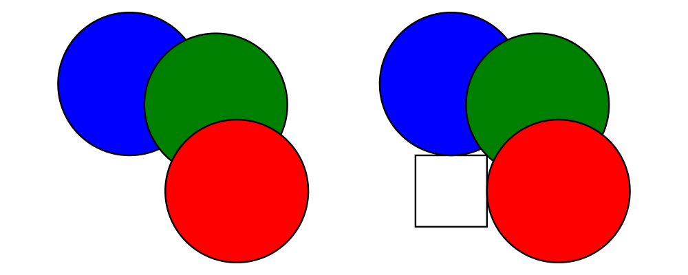
8.1   Calling backends

The simplest way to render a diagram is using either the defaultMain or mainWith functions to generate a default executable that renders the diagram. However, there are other, more flexible ways as well. The precise set of methods available will vary with the particular backend being used, but there are some things that can be said in general.

Many backends provide backend-specific rendering functions. For example, the Cairo backend provides

> renderCairo :: FilePath -> SizeSpec V2 Double -> QDiagram Cairo V2 Double Any -> IO ()

This still causes a rendered diagram to be output to a file, just as in the case of mainWith. The difference is that this is all it does—it is not wrapped inside an executable that expects command-line arguments, and so on. This can be useful if you want a program that does more than just render a single diagram—perhaps it renders multiple diagrams, or perhaps it does things other than just render a diagram, for example, fetch some data over a network and then use the data to generate a diagram which is rendered, and so on.

The most general way to call a backend is to use renderDia, which is a method of the Backend class. Its type (omitting a bunch of type class constraints) is

> renderDia :: (...) => b -> Options b v n -> QDiagram b v n m -> Result b v n

It takes a backend token, an options record, and a diagram, and renders it to some sort of result. Both Options and Result are associated types defined by the Backend class, so what types they actually resolve to depends on the particular backend.

renderDiaT is a variant of renderDia with type

> renderDiaT :: (...) => b -> Options b v n -> QDiagram b v n m -> (Transformation v n, Result b v n)

The only difference is that in addition to a Result, it also returns the Transformation which was generated to transform the given diagram into the coordinates required by the backend (for example, flipping it vertically if the backend's y coordinates increase downwards, resizing and centering to fit the requested dimensions, and so on). The inverse of this transformation can be used to transform output coordinates back into diagram coordinates (for example, in order to map mouse clicks in a GTK window onto a diagram).

8.2   The SVG backend

The SVG backend, diagrams-svg, outputs SVG files. It is the default "out-of-the-box" backend, i.e. what one gets by typing just cabal install diagrams. It is implemented purely in Haskell, with no dependencies on external libraries via the FFI. This means that it should be easy to install on all platforms.

For information on making use of the SVG backend, see Diagrams.Backend.SVG. Gradient support is complete in this backend; however, most browsers do not handle the SVG spec correctly when it comes to reflect and repeat. Apparently only Chrome and IE follow the spec correctly at this point, while Safari does not handle reflect and repeat at all and Firefox gets it wrong.

The SVG backend includes an additional module Diagrams.Backend.SVG.Attributes for SVG specific attributes. Currently the module adds two attributes, SvgId and SvgClass that are used to add class and id to SVG elements. This allows parts of a diagram to be referenced for additional javascript processing when the SVG output is embedded in an HTML file.

The source code for the SVG backend can be found in the diagrams-svg repository. Note the functions renderDia and renderSVG for rendering diagrams directly.

8.3   The Rasterific backend

The Rasterific backend is built on top of the Rasterific package, which is a pure haskell rasterizer that uses JuicyPixels and FontyFruity. This is a fully featured backend that supports the full APi of the diagrams library. It can produce PNG, JPG, BMP, TIF, PDF and animated GIF images. It also supports embedded images (see DImage) and although it does not yet have the text handling capabilities of cairo, it does use the exact text bounding box for alignment. Gradients are fully supported including repetition and reflection. In addition, the Rasterific backend can be used to generate in-memory images that can be manipulated with JuicyPixels. Finally, the Rasterific backend supports grouped opacity.

The Rasterific backend can be invoked via Diagrams.Backend.Rasterific.CmdLine module, or via the renderDia and renderRasterific functions.

8.4   The cairo backend

The cairo backend, diagrams-cairo, is built on top of the cairo package, which contains bindings to the cairo 2D graphics library. Although it is quite full-featured, the cairo library itself can be unfortunately difficult to install on some platforms, particularly OS X.

The cairo backend can produce PNG, SVG, PDF, postscript, and animated GIF output. The cairo backend does support gradients however, due to a bug in the cairo package it does not handle reflect and repeat correctly for radial gradients,

_ `Extend`:http://hackage.haskell.org/package/cairo-0.12.5.3/docs/Graphics-Rendering-Cairo.html#t:Extend

For specific information on how to make use of it, see the documentation for the Diagrams.Backend.Cairo module.

diagrams-cairo was the first officially supported backend, and has

a few advanced features:

  • Diagrams.Backend.Cairo.List exports the renderToList function, which can convert a 2D diagram to a matrix of pixel color values.

  • Diagrams.Backend.Cairo.Ptr exports functions for rendering diagrams directly to buffers in memory.

The source code for the cairo backend can be found in the diagrams-cairo repository. The functions renderDia and renderCairo provide an alternative to the Diagrams.Backend.Cairo.CmdLine interface for more programmatic control of the output.

8.5   The postscript backend

The postscript backend, diagrams-postscript, like the SVG backend, is written purely in Haskell. It outputs encapsulated PostScript (EPS) files. Note that by nature, EPS does not support transparency. The postscript backend also does not support embedded images or gradients. However, it is fairly complete in its support for other features and includes experimental support for multi-page output and CMYK colors.

The source code for the postscript backend can be found in the diagrams-postscript repository.

8.6   The Canvas backend

The Canvas backend is one of the two backends that target the browser. Running a diagram's program that has been compiled using the Canvas backend will create a possibly interactive session accessed at http://localhost:3000/. The Canvas backend is native and uses the blank-canvas package. It is a full featured backend supporting gradients and external images. Diagrams generated with the Canvas backend cannot be saved as graphics files, only as programs to be run locally.

The Canvas backend can be invoked via Diagrams.Backend.Canvas.CmdLine module, or via the renderDia/renderCanvas functions.

8.7   The HTML5 backend

Like the Canvas backend, the HTML5 backend targets the browser. The difference is that the HTML5 backend creates a file of stand alone Javascript and optionally HTML that can be used as a (or part of a) web page. It is based on the static-canvas package. It is a full featured backend supporting gradients and external images.

The HTML5 backend can be invoked via Diagrams.Backend.Html5.CmdLine module, or via the renderDia/renderHtml5 functions.

8.8   The PGF backend

The PGF backend, diagrams-pgf, uses the \(\TeX\) macro package PGF to render diagrams. It supports most features of diagrams including external and (non-transparent) embedded images. Gradients don't support alpha colours and radial gradients' spread methods and positions aren't quite right. These issues will hopefully be fixed in the future.

Since it uses \(\TeX\), it has excellent typographic capabilities, although these require knowledge of \(\TeX\). Simply use the text function to produce text that will be typeset by \(\TeX\). You can also use the text function with a string surrounded by dollar signs ($) to typeset mathematics. The backend also includes experimental functions for querying \(\TeX\) for the size of hboxes, which can be used as a bounding box for a diagram. There are some usage examples in the examples folder of the github page.

The backend can output LaTeX, ConTeXt or plain TeX files (PGF picture code only or standalone TeX files) and can call pdflatex, context or pdftex to make PDF files using texrunner.

8.9   The GTK backend

The GTK backend, diagrams-gtk, used to be part of the cairo backend (and is still built on top of it), but has been split out into a separate package in order to reduce the dependencies of the cairo backend, hence making it easier to install for those who don't need GTK support. You can install it at the same time as the rest of the diagrams framework by passing the -fgtk flag: cabal install -fgtk diagrams, or it can be installed separately later with cabal install diagrams-gtk.

The GTK backend allows rendering diagrams directly to GTK windows instead of to a file (defaultRender and renderToGtk). Note that it is possible to receive mouse clicks and then query the corresponding location in a diagram to find out which part the user clicked on (see Using queries).

The source code for the GTK backend can be found in the diagrams-gtk repository.

8.10   Other backends

For a list of other backends and their status, see the diagrams wiki.

8.11   Tools for backends

  • Diagrams.Segment exports a FixedSegment type, representing segments which do have an inherent starting location. Trails and paths can be "compiled" into lists of FixedSegments with absolute locations using fixTrail and fixPath. This is of interest to authors of rendering backends that do not support relative drawing commands.

  • A test harness for comparing the outputs of different backends can be found in the diagrams-backend-tests repo; the output of the test harness for all officially supported backends is kept up-to-date here.

9   Other tools

There are several "extra" packages which are officially maintained but do not automatically come bundled with the diagrams package.

9.1   diagrams-builder

The diagrams-builder package provides a service for dynamic rendering of diagrams—that is, you hand it a String at runtime representing some diagrams code, and you get back the result of rendering the code using whatever backend you like. This could be useful, for example, as part of a preprocessor tool for interpreting diagrams code embedded in some other document. Currently it is used by the BlogLiterately-diagrams package (for rendering diagrams embedded in blog posts) as well as diagrams-haddock (for rendering diagrams embedded in Haddock comments).

9.2   diagrams-haddock

diagrams-haddock is a tool for embedding diagrams in Haddock documentation. The idea is that you can add images (worth 1000+ words, of course) to your documentation simply by embedding diagrams code in a special format, and then running diagrams-haddock. See the README for instructions on using it.

9.3   SVGFonts

The SVGFonts provides support for reading fonts in SVG format and rendering text to diagrams paths. For more, see Native font support.

10   Type reference

This section serves as a reference in understanding the types used in the diagrams framework.

10.1   Understanding diagrams types

Let's look again at the type of hcat, mentioned in Types and type classes:

> hcat :: (Juxtaposable a, HasOrigin a, Monoid' a, V a ~ V2, N a ~ n, TypeableFloat n)
>      => [a] -> a

This is fairly typical of the types you will encounter when using diagrams. They can be intimidating at first, but with a little practice they are not hard to read. Let's look at the components of this particular type from right to left:

  • [a] -> a. This part is simple enough: it denotes a function from a list of a's to a single a. Typically, the type to the right of => will be some simple polymorphic type.

  • TypeableFloat n. This says that the numeric type n must behave like a real number. TypeableFloat is a type alias for the type families Typeable and RealFloat, which imply Real, Floating, Fractional, Num, and Ord.

  • V a ~ V2, N a ~ n. These are type equality constraints, which say that the types V a and V2 must be equal, and that we will refer to N a with the type variable n. In this case V2 is the type of two-dimensional vectors, and V is a type family which tells us the vector space that corresponds to a particular type. So V a ~ V2 means "the vector space corresponding to a must be two-dimensional", or more informally, "a must be a type representing two-dimensional things".

  • Juxtaposable a, ... These are type class constraints on a, specifying what primitive operations a must support in order to be meaningfully used with hcat. For a complete reference on all the type classes used by diagrams, see the next section, Type class reference.

10.2   Type class reference

This section serves as a reference for all the type classes defined or used by diagrams; there are quite a lot. (Some might even say too many!) Most, if not all, of these are also covered elsewhere, but it is useful to have them collected all in one place. The declaration of each type class is shown along with a short explanation, a list of instances, and links to further reading.

Classes for transforming and combining

HasOrigin

HasOrigin is defined in Diagrams.Core.HasOrigin.

> class HasOrigin t where
>   moveOriginTo :: Point (V t) (N t) -> t -> t

HasOrigin classifies types with a notion of a fixed "location" relative to some "local origin", and provides a means of moving the local origin. This is provided as a separate class from Transformable since some things with a local origin do not support other sorts of transformations; and contrariwise some things that support transformations are translation-invariant (like trails and vectors) and hence do not have a HasOrigin instance.

The moveOriginTo method moves the local origin to the given point.

Instances:

  • The instances for Point, SubMap, Subdiagram, and QDiagram all have the meaning you would expect.

  • The instances for Trace, Envelope, and Query all obey the invariant that, e.g., getEnvelope . moveOriginTo p t == moveOriginTo p t . getEnvelope. That is, if e is the envelope/trace/query for diagram d, moving the origin of e to p yields the envelope/trace/query for d with its origin moved to p.

  • Container types can be translated by translating each element ((a,b), [a], Set, Map).

  • Things wrapped in TransInv are not supposed to be affected by translation, so the TransInv instance has moveOriginTo = const id.

  • The instance for Transformation constructs a translation and composes it appropriately.

Further reading: Alignment.

Transformable

Transformable is defined in Diagrams.Core.Transform.

> class Transformable t where
>   transform :: Transformation (V t) (N t) -> t -> t

It represents types which support arbitrary affine transformations (or linear transformations, in the case of translationally invariant things).

Instances:

  • Prim, SubMap, Subdiagram, QDiagram: these have the meaning you would expect.

  • Of course, Transformation is itself transformable, by composition.

  • Container types can be transformed by transforming each element ((t,t), (t,t,t), [t], Set, Map).

  • Point v n is transformable whenever v n is; translations actually affect points (whereas they might not have an effect on the underlying type v n).

  • Anything wrapped in TransInv will not be affected by translation.

  • Anything wrapped in ScaleInv will not be affected by scaling. See Scale-invariance for more information.

  • Applying a transformation to a Style simply applies it to every attribute.

  • The meaning of transforming an Attribute depends on the particular attribute.

  • The instances for Trace, Envelope, and Query all obey the invariant that, e.g., getEnvelope . transform t == transform t . getEnvelope. That is, if e is the envelope/trace/query for diagram d, transforming e with t yields the envelope/trace/query for d transformed by t.

  • The instance for Deletable simply lifts transformations on the underlying type.

  • The instance for NullPrim does nothing, since there is nothing to transform.

  • Uniform scales can be applied to Double and Rational values; translations can also be applied but have no effect.

Further reading: Euclidean 2-space; 2D Transformations.

Juxtaposable

Juxtaposable is defined in Diagrams.Core.Juxtapose.

> class Juxtaposable a where
>   juxtapose :: Vn a -> a -> a -> a

Juxtaposable represents types of things which can be positioned "next to" one another. Note that this is more general than "having an envelope" (though certainly any instance of Enveloped can be made an instance of Juxtaposable, using juxtaposeDefault). For example, animations are an instance of Juxtaposable (which corresponds to juxtaposing them at every point in time), but not of Enveloped.

juxtapose v a1 a2 positions a2 next to a1 in the direction of v. In particular, it places a2 so that v points from the local origin of a1 towards the old local origin of a2; a1's local origin becomes a2's new local origin. The result is just a translated version of a2. (In particular, juxtapose does not combine a1 and a2 in any way.)

Instances:
  • QDiagram and Envelope are of course instances.

  • Many container types are also instances, since container types have Enveloped instances that work by superimposing all the envelopes of the individual elements: [a], (a,b), Set, Map

Further reading: Juxtaposing diagrams; Juxtaposing without composing.

Enveloped

Enveloped is defined in Diagrams.Core.Envelope. It classifies types which have an associated Envelope.

> class (InnerSpace (V a), OrderedField (N a)) => Enveloped a where
>   getEnvelope :: a -> Envelope (V a) (N a)

The getEnvelope method simply computes or projects out its argument's associated Envelope. InnerSpace, defined in Data.VectorSpace, classifies vector spaces with an inner (dot) product. Computing envelopes almost always involves projection of one vector onto another, which requires an inner product. The OrderedField class is simply a synonym for a collection of classes, requiring that the scalar type have multiplicative inverses and be linearly ordered. See OrderedField.

Instances:
  • The instance for QDiagram does what you would expect.

  • The instance for Subdiagram yields an envelope positioned relative to the parent diagram.

  • Every Point has a "point envelope" consisting of the constantly zero envelope translated to the given point. Note this is not the same as the empty envelope.

  • Many container types have instances which work by combining all the envelopes of the individual elements: [a], (a,b), Set, Map.

Further reading: Envelopes and local vector spaces; Envelopes.

Traced

Traced is defined in Diagrams.Core.Trace, and plays a similar role as Enveloped. Traced types have an associated Trace, which is like an embedded ray tracer that can be used to find points on edges of an object.

> class (Ord (N a), Additive (V a)) => Traced a where
>   getTrace :: a -> Trace (V a) (N a)

Instances:

  • The instance for QDiagram does what you would expect.

  • The instance for Subdiagram yields a trace positioned relative to the parent diagram.

  • The trace of a Point is the empty trace.

  • Many container types have instances which work by combining all the envelopes of the individual elements: [a], (a,b), Set, Map.

Further reading: Traces.

HasQuery

HasQuery is defined in Diagrams.Query, and governs types with an associated Query.

> class HasQuery t m | t -> m where
>   -- | Extract the query of an object.
>   getQuery :: t -> Query (V t) (N t) m

Further reading: Generalized queries.

Classes for attributes and styles

AttributeClass

AttributeClass, defined in Diagrams.Core.Style, is simply a proxy for Typeable and Semigroup; it has no methods. Any type used as an attribute must be made a member of this class.

> class (Typeable a, Semigroup a) => AttributeClass a

Instances: many; see Diagrams.Attributes and Diagrams.TwoD.Path.

Further reading: Attributes and styles; Text.

HasStyle

HasStyle, also defined in Diagrams.Core.Style, classifies things to which a Style can be applied.

> class HasStyle a where
>   applyStyle :: Style (V a) (N a) -> a -> a

applyStyle applies the given Style to an object, combining it on the left with the existing Style (according to the Monoid instance of Style).

Instances:

  • Style itself is an instance.

  • Many container types are instances as long as their elements are; applying a style to a container simply applies the style uniformly to every element: (a,b), Map k a, Set, [a].

  • Functions (b -> a) are an instance as long as a is. (This can also be thought of as a "container type".)

  • Of course, QDiagram b v m is an instance, given a few restrictions on v and m.

Further reading: Attributes and styles; Text.

Classes for names

IsName

IsName is defined in Diagrams.Core.Names. It simply provides the toName method for converting to Name, with a default implementation that wraps up a value as an atomic name. It allows values of arbitrary types to be used as names for subdiagrams.

> class (Typeable a, Ord a, Show a) => IsName a where
>   toName :: a -> Name
>   toName = Name . (:[]) . AName

Instances:

  • Many primitive types such as (), Bool, Char, Int, Float, Double, Integer, String, [a], (a,b), (a,b,c) have a default IsName instance.

  • AName is an instance; converting an atomic name to Name works by creating a singleton list.

  • Name is an instance, with toName as the identity function.

Further reading: Stroking trails and paths; Named subdiagrams; User-defined names.

Qualifiable

Qualifiable is also defined in Diagrams.Core.Names. Instances of Qualifiable are things which can be "qualified" by prefixing them with a name.

> class Qualifiable q where
>   -- | Qualify with the given name.
>   (.>>) :: IsName a => a -> q -> q

Instances:

  • Name: qualifying one name with another is just concatenation.

  • SubMap and QDiagram: qualifying prefixes a name on all the existing names.

Further reading: Named subdiagrams; Subdiagrams; Qualifying names.

Classes for trails and paths

TrailLike

The TrailLike class, defined in Diagrams.TrailLike, abstracts over things that are "trail-like", so that functions such as square can be used to construct a diagram, a path, a trail, etc..

> class (Metric (V t), OrderedField (N t)) => TrailLike t where
>
>   trailLike
>     :: Located (Trail (V t) (N t))  -- ^ The concretely located trail.  Note
>                                     --   that some trail-like things
>                                     --   (e.g. 'Trail's) may ignore the
>                                     --   location.
>     -> t

The trailLike method provides a generic way to build a "trail-like" thing by specifying the low-level trail data. Note that there should usually not be any need for end users to call trailLike directly (though there certainly may be some use cases).

Instances:

  • Trail: this instance simply throws away the location.

  • Trail' Line: throw away the location, and perform cutLoop if necessary. For example, circle 3 :: Trail' Line V2 Double is an open \(360^\circ\) circular arc.

  • Trail' Loop: throw away the location, and perform glueLine if necessary.

  • Path: construct a path with a single component.

  • Diagram b V2 Double: as long as the backend b knows how to render 2D paths, trailLike can construct a diagram by stroking the generated single-component path.

  • [Point v]: this instance generates the vertices of the trail.

  • Located (Trail v), of course, has an instance which amounts to the identity function. More generally, however, Located a is an instance of TrailLike for any type a which is also an instance. In particular, the resulting Located a has the location of the input Located Trail, and a value of type a generated by another call to trailLike. This is most useful for generating values of type Located (Trail' Line v Doubl) and Located (Trail' Loop v). For example, circle 3 # translateX 2 :: Located (Trail' Line V2 Double) is an open \(360^\circ\) circular arc centered at \((2,0)\).

  • Active t (for any TrailLike p): creates a constant Active value.

Further reading: Trails and paths; Trails; Paths; TrailLike.

ToPath

The ToPath class, defined in Diagrams.Path, abstracts over things that can be converted to a Path.

> class ToPath t where
>   toPath :: (Metric (V t), OrderedField (N t))
>          => t -> Path (V t) (N t)

If you have a path, trail, line, loop, etc. with a definite type, you can apply toPath to convert it into a path. A function

> stroke
>   :: ( Renderable (Path V2 (N t)) b, ToPath t
>      , Data.Typeable.Internal.Typeable (N t), RealFloat (N t)
>      , V t ~ V2
>      )
>   => t -> QDiagram b V2 (N t) Any

is also provided, which works by first converting its argument to a Path using toPath, and then calling strokePath on the result. This can be convenient if you have something of a definite type which you want to turn into a diagram; on the other hand, if you have something polymorphic it may be more convenient to use a type-specialized function like strokeLine to fix its type.

Instances:

  • ToPath a => ToPath [a]

  • Trail v n

  • Path v n

  • Located (Trail v n)

  • Located (Trail' l v n)

  • Located (Segment Closed v n)

  • Located [Segment Closed v n]

  • FixedSegment v n

Classes for parametric objects

Diagrams.Parametric provides a set of classes for working with objects which can be viewed as parametric functions, such as segments and trails: Parametric, DomainBounds, EndValues, Sectionable, and HasArcLength. These classes are fairly specialized and do not really show up anywhere else; see the section on Segments and trails as parametric objects for more information.

Classes for backends

Backend

The Backend class, defined in Diagrams.Core.Types, defines the primary interface for any diagrams rendering backend. Unlike many of the other type classes in diagrams, it is quite large. For a full discussion, see the core library reference.

MultiBackend

MultiBackend, also defined in Diagrams.Core.Types, is for backends which support rendering multiple diagrams, for example to a multi-page pdf or something similar. It simply provides the renderDias function for rendering multiple diagrams at once; the meaning of this function depends on the backend.

> class Backend b v n => MultiBackend b v n where
>   renderDias :: (Metric v, OrderedField n, Monoid' m)
>              => b -> Options b v n -> [QDiagram b v n m] -> Result b v n

So far, the only backend which supports multi-diagram rendering is the postscript backend.

Further reading: Rendering backends.
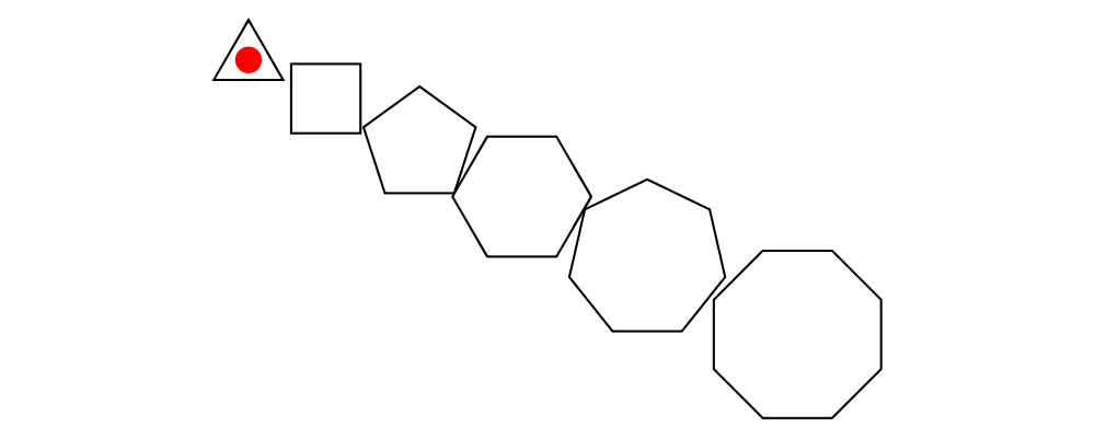
Renderable

The Renderable type class (from Diagrams.Core.Types) is a two-parameter type class connecting backends to primitives which they know how to render. Backend B declares that it knows how to draw primitive P by giving a Renderable P B instance, which requires implementing the render function which takes a primitive and renders it.

> class Transformable t => Renderable t b where
>   render :: b -> t -> Render b (V t) (N t)

Instances: There are many instances defined by each backend.

Further reading: Rendering backends.
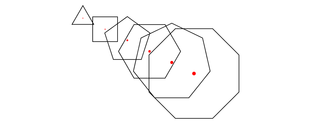
ToResult

The ToResult class (from Diagrams.Backend.CmdLine) essentially defines a very generic form of uncurrying. It is used to implement the general interface for building command-line-driven diagram generation programs, and in particular to enable building executables out of (curried) functions, which requires collecting up all their arguments at once. See the command-line tutorial for more.

> class ToResult d where
>     type Args d :: *
>     type ResultOf d :: *
>
>     toResult :: d -> Args d -> ResultOf d

The most interesting instance is the one for functions:

> instance ToResult d => ToResult (a -> d) where
>     type Args (a -> d) = (a, Args d)
>     type ResultOf (a -> d) = ResultOf d
>
>     toResult f (a,args) = toResult (f a) args

Parseable

The Parseable class (Diagrams.Backend.CmdLine) contains just one method, parser :: Parser a, which defines a command-line parser for a given type. Things with Parseable instances can be used in conjunction with the command-line creation framework. See the command-line tutorial for more.

Mainable

The Mainable class (Diagrams.Backend.CmdLine) governs types which can be used to build a command-line-driven diagram-generation program. For example, a diagram; but also animations, lists of diagrams, association lists of strings and diagrams, and functions from parseable things to any of the above. See the command-line tutorial for more.

> class Mainable d where
>     type MainOpts d :: *
>
>     mainArgs   :: Parseable (MainOpts d) => d -> IO (MainOpts d)
>     mainRender :: MainOpts d -> d -> IO ()
>     mainWith   :: Parseable (MainOpts d) => d -> IO ()

Poor man's type synonyms

There are several cases where a certain set of type class constraints are used together so often that it is convenient to define a synonym to stand in for the entire set of constraints. In more recent versions of GHC that support the ConstraintKinds extension, this could be accomplished with a simple type synonym. However, since diagrams still supports older versions of GHC, these are declared as a new type class with no methods and a single universal instance. For example,
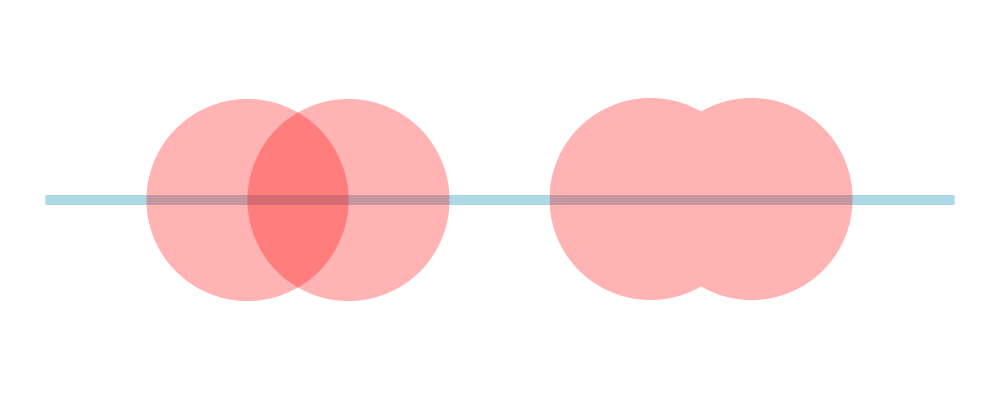
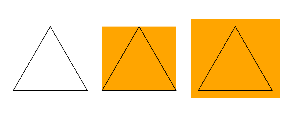
> class (Class1 a, Class2 a, Class3 a) => Synonym a
> instance (Class1 a, Class2 a, Class3 a) => Synonym a

Ideally, at some point in the future diagrams will drop support for versions of GHC without ConstraintKinds and switch to the more sensible way of defining constraint synonyms.

Monoid'

Monoid' m is a synonym for

(Semigroup m, Monoid m),

defined in Diagrams.Core. This is something of an unfortunate hack: although every monoid is a semigroup mathematically speaking, Semigroup is not actually a superclass of Monoid, so if we want to use both we have to actually declare both.

HasBasis

HasBasis v is a synonym for

(Representable v, Rep v ~ E v),

which is used to get access to the basis elements of a vector.

HasLinearMap

HasLinearMap v is a synonym for

(Additive v, Applicative v, Traversable v),

which is used for many of the functions related to transforms.

OrderedField

OrderedField s, defined in Diagrams.Core.Envelope, is a synonym for

(Floating s, Ord s),

i.e. a floating-point type which is totally ordered. When dealing with Envelopes it's often necessary to have scalars which support all four arithmetic operations as well as square root, and can be compared for ordering.

TypeableFloat

TypeableFloat n, defined in Diagrams.Core.Types, is a synonym for

(Typeable n, RealFloat n)

which implies (Real n, Floating n, Fractional n, Num n, Ord n). These constraints are needed on many functions that produce diagrams, due to constraints on transformations and attributes.

DataFloat

DataFloat n is the same as TypeableFloat n, but strengthens the Typeable constraint to Data.

InSpace

InSpace v n a is a synonym for (V a ~ v, N a ~ n, Additive v, Num n). That is, the type a belongs to the vector space v n, where v is Additive and n is a Num.

SameSpace

SameSpace a b is a synonym for (V a ~ V b, N a ~ N b), that is, the types a and b belong to the same vector space v n.

10.3   Type family reference

Type families are a GHC extension to Haskell enabling "type-level functions". You can read about them in detail here, but understanding them enough to use them as they arise in diagrams is not anywhere near as complicated as that page might suggest. Simply put, type families are functions which can take types as input and produce other types as output. Of course, in one sense any polymorphic type constructor already does this: for example, Maybe takes types as input (say, Int) and produces types as output (say, Maybe Int). The difference is that Maybe works uniformly for all input types (it does not, indeed cannot, do anything "different" for Char than it does for Int). Type families, on the other hand, can have a specific definition for each input type (much as type class methods can have a different implementation for each instance type). For example, the following (admittedly contrived) example declares a type family named Foo, with two definition clauses.

> type family Foo a :: *
> type instance Foo Int  = Int
> type instance Foo Char = [String]

Diagrams only makes use of a few type families, though two of them (V and N) are used quite extensively. The following sections list each of the type families employed by diagrams.

V

The V type family is defined in Diagrams.Core.V. The idea is that many types have an "associated" vector space, i.e. the vector space in which they "live". The vector space is described by its dimension and its numeric type. V simply maps from types to a type representing the vector space dimension. For example, V (Path V2 Double) = V2 (ordinary two-dimensional paths live in V2 Double), and V [a] = V a (lists of a's live in whatever vector space a's themselves live in).

Often, V shows up in a constraint on the left hand side of =>, as in

> alignT :: (Alignable a, HasOrigin a, V a ~ V2, N a ~ n, Floating n) => a -> a

This type says that alignT can be applied to values of any type a, as long as a is an instance of Alignable, and a lives in the vector space V2, that is, V a ~ V2 (the tilde expresses a type equality constraint).

Other times, V can show up on the right-hand side of =>, as in

> deform :: Deformation (V a) (N a) -> a -> a

This says that deform takes two arguments: a Deformation and a value of some type a. However, Deformationss are parameterized by a vector space; Deformation (V a) (N a) means that the vector space of the deformation is the vector space associated to a. Many types in diagrams are parameterized this way, by v and n parameters which together define a vector space.

N

The N type family is defined in Diagrams.Core.V. Whereas V describes the dimension of a vector space, N describes the scalar value used to represent coördinates or distances in the space. A "scalar" can be thought of as a distance, or scaling factor. For example, you can scale a vector by a scalar (using (*^)), and the norm function takes a vector and returns a scalar.

Vn

Vn is a type synonym yielding a common combination of V and N:

> type Vn a = V a (N a)

That is, Vn a is the type of a concrete vector space associated to a, obtained by extracting the vector space dimension V a and applying it to the type of scalars N a.

Render

Render is an associated data family of the Backend class. It determines the type of rendering operations for a given backend. For more information, see the core library reference.

Result

Result is an associated type family of the Backend class. It determines the type of the final result obtained from the backend after rendering a complete diagram. For more information, see the core library reference.

Options

Options is an associated data family of the Backend class. It determines the type of options which can be passed to the backend when initiating a rendering operation. For more information, see the core library reference.

Codomain

Codomain is a type family defined in Diagrams.Parametric. Parametric objects of type a can be viewed as functions of type N a -> Codomain a. For more information, see Segments and trails as parametric objects.